Structural topology optimization considering temperature dependent Young’s modulus of polymersc

Seongwon Bae; Sunghoon Lim; Kozo Furuta; Kazuhiro Izui; Shinji Nishiwaki

doi:10.7776/ASK.2026.45.2.149

Preview

Research Article

The Journal of the Acoustical Society of Korea. 31 March 2026. 149-162
https://doi.org/10.7776/ASK.2026.45.2.149

Structural topology optimization considering temperature dependent Young’s modulus of polymers

온도에 따라 변화하는 고분자의 영률을 고려한 구조 위상 최적화에 관한 연구

Seongwon Bae¹^*

Sunghoon Lim²

Kozo Furuta²

Kazuhiro Izui²

Shinji Nishiwaki²

배 성원¹^*

임 성훈²

후루타 코조²

이주이 카즈히로²

니시와키 신지²

¹ES Laboratory LG Electronics

²Kyoto University

^{*Corresponding Author}

License (open-access, http://creativecommons.org/licenses/by-nc/4.0/):

This is an Open Access article distributed under the terms of the Creative Commons Attribution Non-Commercial License which permits unrestricted non-commercial use, distribution, and reproduction in any medium, provided the original work is properly cited.

ABSTRACT

Polymers, along with metals, are most widely used as structural materials for air conditioners. Polymers are lightweight and have low thermal conductivity, so they are used to protect customers from hot or cold surfaces, reduce weight, and improve appearance. However, structural properties such as the Young’s modulus of the polymer are temperature dependent, which changes significantly as it approaches the melting point or glass transition temperature. Operating the air conditioner for winter heating can heat-deform the polymer and cause loud squeaking noise due to friction deformation motion. To solve this problem, Young’s modulus, which depends on temperature, is expressed as a simplified function and a topology optimization model using it is proposed. In addition, the usefulness is demonstrated by performing structural phase optimization for static and dynamic problems and multi objective problems with both items using this model.

Keywords

Heat dependant Young’s modulus

Dynamic compliance minimization

Rattling noise

Polymer

Thermoelasitc

Air conditioner

폴리머는 금속과 함께 에어컨의 구조 재료로 가장 널리 사용되는 소재입니다. 고분자 물질은 가볍고 열전도도가 낮으며 외관이 반짝이는 특성이 있어서, 뜨겁거나 차가운 표면으로부터 고객을 보호하고 제품의 무게를 줄이며 외관을 개선하는 데 사용됩니다. 그러나 이 고분자는 소재의 온도가 녹는점이나 유리화 온도에 가까이 가는 등 온도 변화가 심할 때 온도에 따라 영률과 같은 구조적 물성이 변화합니다. 겨울철 난방을 위해 에어컨을 가동하면 폴리머가 열에 의해 변형되고 상대적 변형에 의한 마찰 운동에 의해 삐걱거리는 소음이 크게 발생할 수 있습니다. 이 문제를 해결하기 위해 온도에 따라 달라지는 영률을 단순화된 함수로 표현하고 이를 이용한 토폴로지 최적화 모델을 제안합니다. 또한, 이 모델의 유용성을 보이기 위하여 정적 및 동적 문제 그리고 두 문제를 혼합한 다목적 문제에 대한 구조적 위상 최적화를 수행하였습니다.

키워드

온도 의존적 영률

동적 컴플라이언스 최소화

래틀링 소음

고분

열탄성

에어컨

MAIN

I. Introduction
II. Formulation
2.1 Temperature dependent Young’s modulus
2.2 Thermoelasticity problem
2.3 Dynamic problem
2.4 Temperature field
2.5 Optimization problem formulation
2.6 Optimization algorithm
III. Numerical examples
3.1 Rectangular model
3.2 A Vane of heat pump model
IV. Conclusion

I. Introduction

Polymers are most widely used as structural materials for air conditioners to reduce product weight and protect customers from heat and electrical hazards caused by mechanical products. Despite these advantages, polymer parts are also a frequent cause of customer complaints due to deformed appearances or rattling noises. One of the most critical reasons for this difficulty in design is the complex mechanical material properties of polymers compared to metals. For example, Young’s modulus, essential for structural design, is often expressed as a curve or range. Depending on whether the polymer is thermoplastic or thermosetting, the pattern of the characteristic curve changes completely, and the values of mechanical properties can vary rapidly or slowly depending on environmental conditions such as temperature changes, humidity, and ozone exposure near the ocean.

When designing mechanical products using polymers, their mechanical properties are most rapidly affected by internal or external temperature changes. Among the properties of structural materials, the most pressing issue to solve is the temperature dependent Young’s modulus. For instance, when operating a heat pump in winter, the temperature of some structures may fluctuate by more than 100 °C within a few minutes. This can cause visible deformation of the product. Additionally, noise may arise from changes in resonance frequency or rattling between parts with differing thermal expansion coefficients.^[1,2]

When this problem was first identified, improved polymer materials is applied to reduce thermal deformation. Carbon fiber was added and engineering plastics were also considered. However, these solutions were not adopted for manufacturing because of little improvement in thermal deformation compared to cost increases. Recently, the technology of inserting air bubbles has been widely applied. While this approach prevents cost increases, it is difficult to use for exterior materials because the air bubble mark is visible on the surface.

Next, efforts were made to modify the structural design using finite element method. The first step involved measuring the complex properties of polymers, followed by applying thermoelastic analysis using temperature field measurement results. When the polymer property graph could not be directly applied to the analysis model, a segmented model was used to specify properties for each temperature range. Vibration analysis was also performed in the same manner. Afterward, trial and error iterations were repeated to derive improved results.

Nowadays, topology optimization has been introduced and has become a highly effective method for reducing trial- and-error processes in the air-conditioner industry. Topology optimization methods for thermoelastic and frequency response problems are widely used to solve such structural design challenges.

The first method, topology optimization for thermoelastic problems, has a long history. Rodrigues et al. introduced a material based model for topology optimization of thermoelastic structures.^[3] They performed compliance minimization with a volume constraint while considering both thermal and mechanical loads. Li et al. introduced thermoelastic topology optimization using Evolutionary Structural Optimization (ESO), accounting for nonuniform temperature distribution, multiple thermal loads, and transient heat conduction fields.^[4] Xia et al. studied the application of the level set method to thermoelastic problems to reduce gray-scale elements in the solution.^[5] Gao et al. introduced thermal stress coefficients and ramped models to provide more stable iterations.^[6] Chung et al. studied nonlinear thermoelasticity using the level set method.^[7] More recently, Chen et al.^[8] and Zheng et al.^[9] studied thermoelastic problems considering temperature dependent material properties in 2022 and 2023, respectively.

The second method involves research on minimizing dynamic compliance, introduced by Ma et al.^[10] The study on transient problems was demonstrated by Min et al.^[11] Later, Olhoff et al.^[12] identified mechanisms for minimizing dynamic compliance by increasing or decreasing natural frequencies. However, because a large number of gray scale elements are generated during optimization when decreasing natural frequencies, studies using the level set method were introduced by Shu et al.^[13] to reduce them. Additionally, Silva et al.^[14] addressed problems where the exit region and fixed boundary are not connected. It’s hard to find a paper on the minimization of dynamic compliance by temperature dependent mechanical material properties. The measurement and simulation of Young’s modulus according to polymer temperature are well documented in polymer chemistry textbooks and papers.^[15,16,17] Recently, it has become possible to predict Young’s modulus based on the combination of bonding forces in polymer chemistry.^[17] Therefore, if topology optimization technology using temperature dependent Young’s modulus is available, it becomes possible to perform topology optimization of structures using new polymer materials.

In this paper, research is conducted utilizing the temperature dependent Young’s modulus of thermoplastic materials among these polymers. However, the damping coefficient is also temperature dependent due to its viscoelastic characteristic, but it is ignored. Because the behavior near the resonance point is not the focus, and the contents become too complicated. Therefore, the clear limitations of this study should be considered. A Young’s modulus is expressed as a function of temperature and is applied to topology optimization for thermoelastic problems, dynamic compliance minimization, and multi-objective optimization that combines both. The temperature distribution is calculated using the steady state thermal conduction function, and since nonlinear effects are minimal in both thermal conduction and thermoelastic problems, they are computed serially using linear equations. Optimization results are derived using the density method, reaction diffusion equation, and adaptive meshing techniques to reduce gray scale elements. In addition, when multi objective topology optimization is applied, it is analyzed whether a solution is derived from the loading point to the boundary at the excitation frequency where many gray scaled elements are derived. The focus of this paper is the trend of shape change and compliance change of the solution, and detailed stress concentration that can be applied directly to actual mass production is not considered.

II. Formulation

2.1 Temperature dependent Young’s modulus

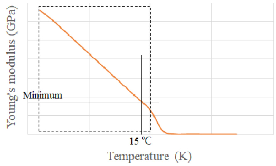
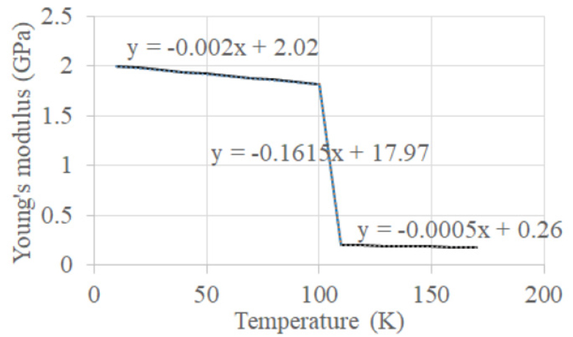
The Young’s modulus pattern according to the temperature of the amorphous thermoplastic polymer is shown in Fig. 1^[15,16,17]. In case of the slope in Fig. 1(a), the polymer structure is not changed and the Young’s modulus is reduced by temperature, and the slope can be relatively gentle and steep cases depending on the material. Fig. 1(b) is a type that maintains a similar Young’s modulus when the temperature is lower than the glassy temperature, but drops sharply when the temperature is higher than the glassy temperature. While most designs are performed in the left box area shown in Fig. 1(a), structural designs are also performed in the area of the right box to ensure safety. In this paper, the complex Young’s modulus curve in Fig. 1 is simplified for each section as shown in Fig. 2 and formulated as a linear function.

https://cdn.apub.kr/journalsite/sites/ask/2026-045-02/N0660450205/images/ASK_45_02_05_F1.jpg

Fig. 1.

General Young’s modulus pattern of the amorphous (a) and reinforced amorphous (b) polymer.

https://cdn.apub.kr/journalsite/sites/ask/2026-045-02/N0660450205/images/ASK_45_02_05_F2.jpg

Fig. 2.

Approximated Young’s modulus pattern of the amorphous polymers.

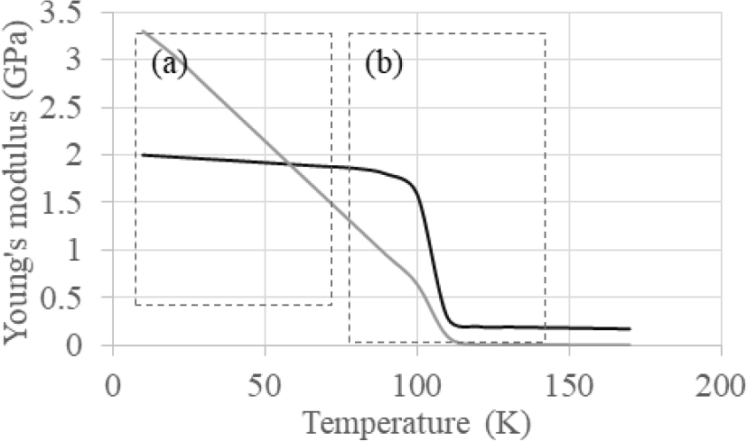
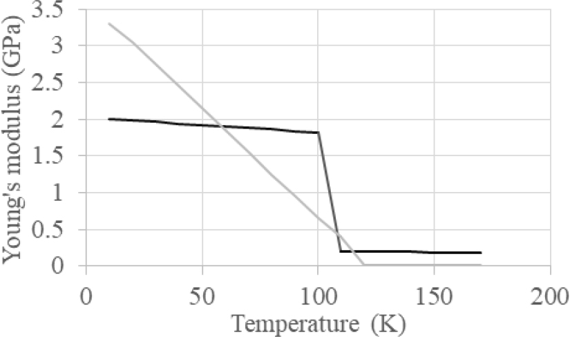
Using the linear expression of the three sections is the closest to the original curve even compared to the sixth- order polynomial, exponential, and logarithmic functions, so the linear expression of the three sections is used. Young’s modulus (E) by temperature (t) are defined as follow:

(1)

E (t) = (C_{1} t + C_{2}) E_{0},

where $E_{0}$ , $C_{1}$ and $C_{2}$ are young’s modulus on initial temperature $t_{0}$ and two linearized coefficients.

2.2 Thermoelasticity problem

Variational formulation for thermoelasticity problem is defined in analysis domain (𝛺) as follows^{[3,4,5,6,7,8,9]}:

(2)

\int_{Ω} E_{i j k l} ε_{k l} (u)_{ε_{i j}} (v) d Ω = \int_{Ω} E_{i j k l} ε_{k l}^{t} (u)_{ε_{i j}} (v) d Ω + \int_{Ω} f ∙ v d Ω,

where u, v and f are displacement vector, test function, and force vector. Deformation tenser $ε_{i j}$ , elasticity tensor $ε_{k l}^{t}$ , thermal strain $ε_{k l}^{t}$ and Lame´ coefficients are defined as follows

(3)

ε_{i j} = \frac{1}{2} (\frac{\partial u_{i}}{\partial x_{j}} + \frac{\partial u_{j}}{\partial x_{i}}),

Here,

(4)

σ_{i j} = E_{i j k l} (ε_{k l} - ε_{k l}^{t}),

(5)

ε_{k l}^{t} = α Δ T δ_{k l},

(6)

E_{i j k l} = λ δ_{i j} δ_{k l} + μ (δ_{i k} δ_{j l} + δ_{i l} δ_{j k}),

(7)

μ = \frac{E}{2 (1 + ν)}, λ = \frac{E ν}{(1 - 2 ν) (1 + ν)},

where T and α are temperature and isotropic heat transfer coefficient. The Young’s modulus E(t) are defined in terms of element density ( $x_{e}$ ) as follow:

(8)

E = x_{e}^{p} (E (t) - E_{\min}) + E_{\min},

where $E_{\min}$ is the minimum Young’s modulus which is defined in void region to prevent a singularity problem. p is a penalization factor of which the value is set to 3 in this study.

2.3 Dynamic problem

The variational formulation of the harmonic vibration problem is expressed in the analysis domain (𝛺) as follows^{[10,11,12,13,14]}:

(9)

\frac{\partial^{2}}{\partial t^{2}} ρ \int_{Ω} u v d Ω + \int_{Ω} 2 μ e (u) ∙ e (v) d Ω + \int_{Ω} λ d i v (u) d i v (v) d Ω = \int_{Ω} f ∙ v d Ω,

where ρ is density, µ and λ are Lame´ coefficients of homogeneous isotropic material. It’s noted that damping terms are not considered in the governing equation. u, v, and f are displacement vector, test function, and force vector, respectively. Deformation tenser (e) is defined as follows:

(10)

e (u) = \frac{1}{2} (\nabla u + \nabla u^{T}) .

2.4 Temperature field

Weak form of temperature field^[18] assuming steady state can be expressed using Laplacian function as follows:

(11)

\int_{Ω} α \nabla T ∙ \nabla v = \int_{Ω} Q ∙ v d Ω,

where Q is a internal heat and no internal heat source is used in this paper.

The thermal stress and temperature fields are weakly coupled. However, they are not dominant compared to other factors, so they are considered independently in the process of calculating the sensitivity.

2.5 Optimization problem formulation

2.5.1 Thermoelastic problem

The optimization problem formulation to minimize compliance of thermoelastic problem is well known as follows^{[3,4,5,6,7,8,9]}:

(12)

minimize Φ_{t} = C_{t} = \int_{Ω} E_{i j k l} ε_{k l}^{t} (u)_{E_{i j}} (v) d Ω + \int_{Ω} f ∙ v d Ω, subject to \int_{Ω} x_{e} d Ω / \int_{Ω} d Ω \leq V_{f},

where ( $V_{f}$ ) is upper limit of volume fraction. The Lagrangian (F) of objective function is expressed as follows:

(13)

minimize F = Φ (x_{e}) + γ (\int_{Ω} x_{e} d Ω - V_{f} \int_{Ω} d Ω) .

The sensitivity also well known as follows:

(14)

\frac{\partial F}{\partial x_{e}} = \frac{\partial}{\partial x_{e}} \int_{Ω} (2 E_{i j k l} ε_{k l}^{t} (u)_{ε_{i j}} (v) - E_{i j k l} ε_{k l} (u)_{ε_{i j}} (v)) d Ω + γ .

2.5.2 Dynamic problem

In order to reduce the frequency response of a structure, dynamic compliance ( $C_{d}$ ) is defined as the objective function to be minimized. This is expressed as follows^[10]:

(15)

Minimize Φ_{d} = C_{d} = |U (ω)^{T} F (ω)| subject to \int_{Ω} x_{e} d Ω / \int_{Ω} d Ω \leq V_{f} .

To solve the above constrained optimization problem, unconstrained problem using Lagrangian for dynamic problem is defined as follows:

(16)

minimize L (x_{e}) = \bar{Φ_{d}} (x_{e}) + γ (\int_{Ω} x_{e} d Ω - V_{f} \int_{Ω} d Ω),

where γ is Lagrange multiplier for satisfying volume fraction constraint.

The sensitivity for dynamic problem is expressed as follows:

(17)

\frac{\partial L}{\partial x_{e}} = \frac{\partial}{\partial x_{e}} \int_{Ω} (- j ω^{2} ρ u v d Ω + 2 μ e (u) ∙ e (v) + λ div (u) div (v)) d Ω + γ .

2.5.3 Multi objective problem

The multi objective function composed of thermoelastic and dynamic compliance as follows:

(18)

\bar{Φ_{m}} = η C_{t} + (1 - η) C_{d},

where η is a weighting factor.

2.5.4 Augmented Lagrangian for inequality constrained problem

Augmented Lagrangian method is used to convert from constraint to unconstrained optimization problem. From Eq. (12), volume constraint can be expressed as follows^[19]:

(19)

G (x_{e}) = \frac{\int_{Ω} x_{e} d Ω}{\int_{Ω}^{\cdot} d Ω} - V_{f} = \frac{\int_{Ω} x_{e} d Ω}{| Ω |} - V_{f} \leq 0,

Augmented Lagrangian $\tilde{F}$ and Lagrangian multiplier $G^{i + 1}$ are defined as follows:

(20)

\tilde{F} = η Φ (x_{e}) + G^{i + 1},

where $η = \frac{| Ω |}{||d F / d x_{e}|| L^{2} (Ω)}$

(21)

G^{i + 1} (x_{e}) = q G^{i} (x_{e}) + \frac{1}{2} r G^{i^{2}} (x_{e}), if G \geq - \frac{q}{r} G^{i + 1} (x_{e}) = - \frac{q^{2}}{r}, if G \leq - \frac{q}{r},

where a positive scalar q and r are the Lagrange multiplier for the inequality constraint and the penalty factor. η is a normalization factor.

2.5.5 Reaction Diffusion Equation (RDE)

There are two update scheme to reduce calculation time and gray-scale elements in this paper. First, Reaction Diffusion Equation (RDE) using fictitious time (t) is applied for first stage. RDE in design domain (𝛺) and the boundary (∂𝛺) is defined as follows^[20,21]:

(22)

\frac{\partial x_{e}}{\partial t} = κ \nabla^{2} x_{e} - \frac{\partial \tilde{F}}{\partial x_{e}}, in Ω,

(23)

\frac{x_{e}}{n} = 0, on \partial Ω,

where κ is a diffusion coefficient.

Second, RDE integrated with Double-Well Potential (DWP) is used to reduce gray-scale element in second stage. RDE with DWP is defined as follows:

(24)

\frac{\partial x_{e}}{\partial t} = κ \nabla^{2} x_{e} - \{a w^{'} (x_{e}) + 30 w (x_{e}) \frac{\partial \tilde{F}}{\partial x_{e}}\} in Ω,

(25)

\frac{x_{e}}{n} = 0, on \partial Ω,

where $w (x_{e}) = x_{e}^{2} (1 - x_{2})^{2}$ , a are smooth Dirac delta function and control parameter for the thickness of gray-scaled zone.

2.6 Optimization algorithm

The optimization algorithm consists of two steps, as shown in Fig. 3. The first step is a quick computational step using smaller elements and RDE update schemes. The second step is a gray scale reduction step using adaptive mesh and DWP update schemes. The reasons to use a two step algorithm is to obtain lower gray scale elements and calculation time. In the case of this paper’s problem, the result of updating about 3,000 Time (s) using RDE alone and the result of mixing RDE 300 s + Adaptive mesh 50 s are similar, but it is not a major issue, so it is omitted.

https://cdn.apub.kr/journalsite/sites/ask/2026-045-02/N0660450205/images/ASK_45_02_05_F3.jpg

Fig. 3.

Total optimization flow.

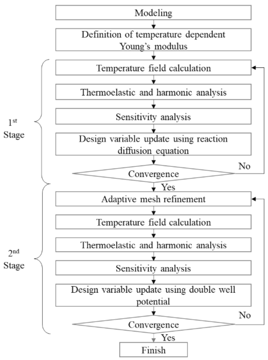
If only RDE is used for the update scheme, a large amount of gray scale elements are generated in the diffusion term of the RDE and more iterations are required to reduce the gray scale elements and to achieve clear boundary. When using only adaptive mesh refinement for updates, more elements are used, which takes more time to calculate. Therefore, a two step computation procedure can lead to results with fewer gray scale elements and less computation time. In this paper, the adaptive mesh refinement algorithm of FreeFEM++ is used for calculations.

III. Numerical examples

3.1 Rectangular model

3.1.1 Thermoelastic problem

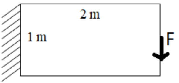
A Rectangular model is used for an example as Fig. 4. Young’s modulus (E₀), Poisson ratio (ν), and heat expansion ratio (α) are 199.5 (MPa), 15.4 × 10^–6 (/K) and 0.3 as a sample problem. The loaded force (F), target volume fraction and thermal conductivity coefficient are 10,000 (N), 0.2 and 0.13 (W/mK). The optimized results with uniform temperature distribution are shown in Fig. 5. Compliance with each initial condition is shown in Table 1. All trends of these results in Fig. 5 and Table 1 are same as the result in References [10, 11, 12, 13, 14]. The same volume fraction is used, but it is found that a solution with less volume is derived with increasing temperature. This means that the solution is derived in the direction of decreasing density because the direction of the sensitivity function of the thermo-elastic term is opposite to that of the elastic term. In addition, as shown in Table 1, compliance without thermal loading is 37.38 J, which means that thermal load is the dominant factor compared to static load.

https://cdn.apub.kr/journalsite/sites/ask/2026-045-02/N0660450205/images/ASK_45_02_05_F4.jpg

Fig. 4.

Rectangular model.

https://cdn.apub.kr/journalsite/sites/ask/2026-045-02/N0660450205/images/ASK_45_02_05_F5.jpg

Fig. 5.

Optimized result using uniform temperature.

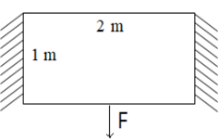
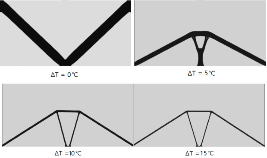
Table 1.

Compliance and $V_{f}$ in uniform temperature.

∆T	0 °C	5 °C	10 °C	15 °C
Compliance initial	37.38	636.45	1919.34	4452.54
Compliance after	0.22	1.53	3.68	5.50
Volume fraction	0.19	0.10	0.05	0.03

The optimized results with two non-uniform temperature distribution cases are introduced in Fig. 6 but the Young’s modulus are not changed to compare. The maximum temperature change of the models is 15 °C and the minimum is 0 °C. From the results in Fig. 6, it is found that the overall shape is similar, but the distribution of the material is different. In order to maintain the stiffness in the same volume, the volume of the low temperature part where Young’s modulus is high increases, and in order to reduce the stress caused by thermal expansion, a solution in which the material is reduced in the high temperature part is derived. The effect of temperature distribution on compliance is shown in Tables 1 and 2 when the E₀ ratio is the same in case 1 and when the E₀ ratio is homogeneously increased by 15℃ degrees. Since the overall heat load of case 1 is less than that of the uniform load, compliance is about 5 % small.

https://cdn.apub.kr/journalsite/sites/ask/2026-045-02/N0660450205/images/ASK_45_02_05_F6.jpg

Fig. 6.

Optimized results using non uniform temperature.

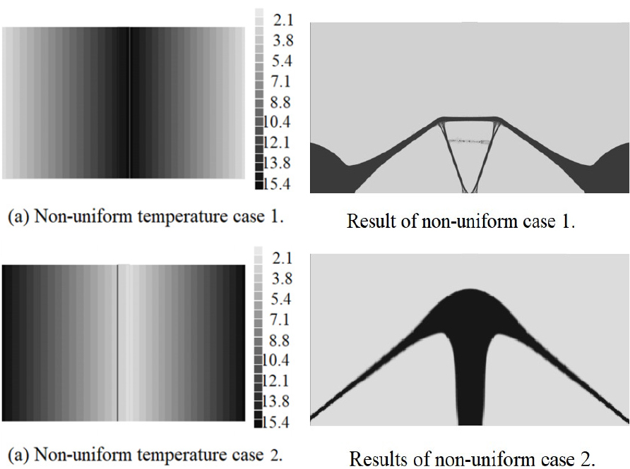
Table 2.

Compliance and $V_{f}$ in temperature case 1.

E₀ ratio	0	0.5	0.1	0.01
Compliance	5.21	5.21	26.93	108.87
Volume fraction	0.11	0.12	0.18	0.18

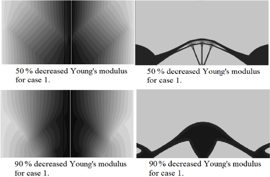
To see the effect of temperature dependent Young’s modulus, a linear model is applied for cases 1 and 2 like Fig. 7. The example cases of temperature dependent Young’s modulus are 50 %, 90 % and 99 % reduction like Fig. 8 and 9. for cases 1 and 2 in Fig. 6.

https://cdn.apub.kr/journalsite/sites/ask/2026-045-02/N0660450205/images/ASK_45_02_05_F7.jpg

Fig. 7.

(Color available online) Temperature dependent Young’s modulus model 1.

https://cdn.apub.kr/journalsite/sites/ask/2026-045-02/N0660450205/images/ASK_45_02_05_F8.jpg

Fig. 8.

Effects of decreased Young’s modulus using case 1. without temperature updating.

https://cdn.apub.kr/journalsite/sites/ask/2026-045-02/N0660450205/images/ASK_45_02_05_F9.jpg

Fig. 9.

Effects of decreased Young’s modulus using case 2. without temperature updating.

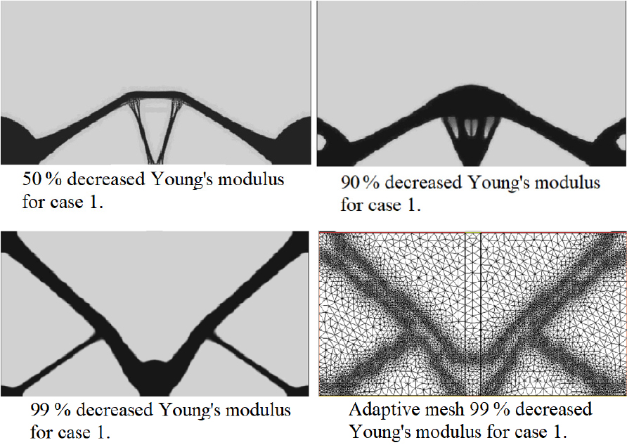
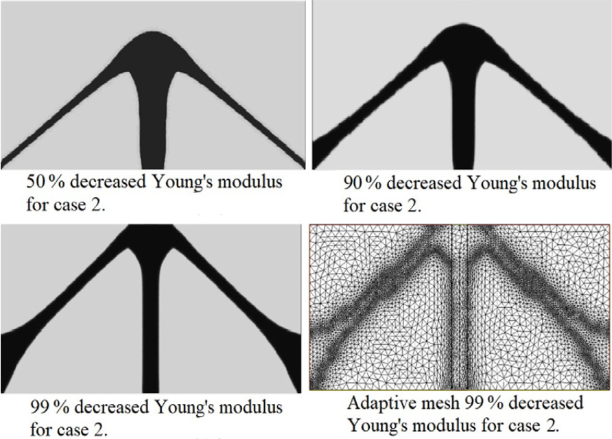
In the result in Fig. 8, the temperature of central area the highest and Young’s modulus become the lowest. The mass in central area become larger and it’s opposite direction from the cases in Fig. 6. Because the Young’s modulus become reduced, thermostatic load become reduced in high temperature area. This trend is shown with similar trend in Fig. 9. It’s shown that the Young’s modulus reduction with temperature become larger, the compliance is also increased in Table 2. Compliance in case 2 is shown in Table 3, and lower compliance results are achieved compared to case 1. When E₀ is 0, the difference of thermal load in two cases is shown, and the trend of compliance is also different when the temperature dependent Young’s modulus decreases. It means that static load and thermal load are differently affected in the process of deriving the solution of the two cases.

Table 3.

Compliance and $V_{f}$ in case 2.

E₀ ratio	0	0.5	0.1	0.01
Compliance	0.77	1.32	5.55	68.59
Volume fraction	0.15	0.15	0.18	0.19

From these result. it’s expected the optimized design for metal and polymer components can be different way and the temperature dependent of Young’s modulus must be considered for polymers or such a materials.

In next, the change of temperature with changed volume is considered because the heat dependent Young’s modulus is applied for the optimization. The temperature field is updated as Fig. 3 without coupled mechanical model. Because it’s considered that heat transfer and thermostatic problem are coupled weakly and when the number of iteration is enough, the result will be converged or slightly different with coupled results. It’s modeled that temperature of hottest and lowest area are specified and the distribution of temperature is updated using heat transfer coefficient using changed density. The optimization results of case 1 are presented in Fig. 10.

https://cdn.apub.kr/journalsite/sites/ask/2026-045-02/N0660450205/images/ASK_45_02_05_F10.jpg

Fig. 10.

Result of updated temperature field in case 1.

Trend of those results are same as former cases. When the Young’s modulus is decreased, the density become increased in hot area. However, influence of density distribution is smaller than Young’s modulus.

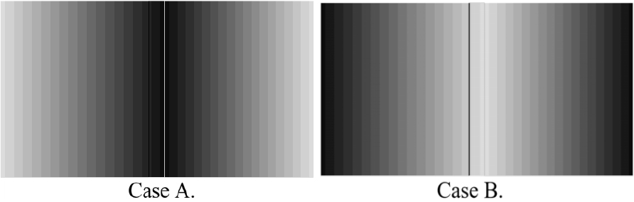
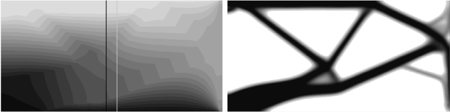
An additional example is introduced to compare the effects on different temperature distribution and the results of the change in the ratio of static and thermal loads with same rectangular model in Figs. 11 and 12. The force is veried from 10⁴ N to 10⁵ N and frequency of 1 Hz and 60 Hz are used for calculation. The function of 90 % decreased Young’s modulus by 15 °C increased temperature is used.

https://cdn.apub.kr/journalsite/sites/ask/2026-045-02/N0660450205/images/ASK_45_02_05_F11.jpg

Fig. 11.

Temperature distribution cases.

https://cdn.apub.kr/journalsite/sites/ask/2026-045-02/N0660450205/images/ASK_45_02_05_F12.jpg

Fig. 12.

Effect of increased load forces using thermal case B.

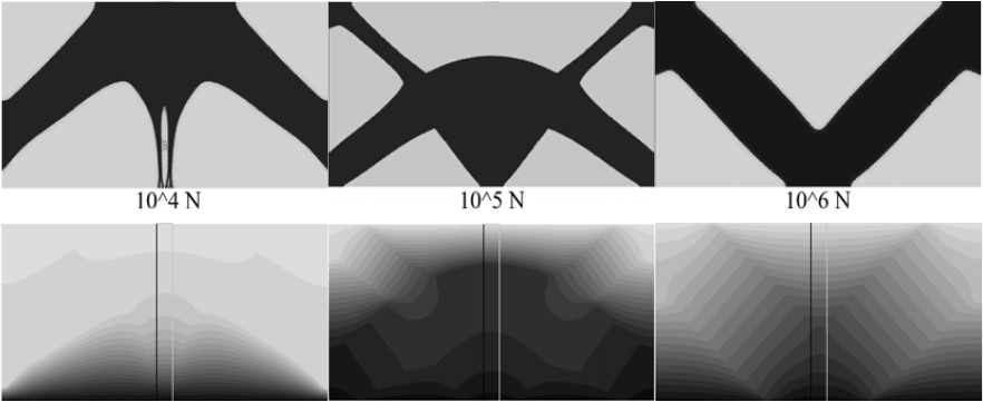
In the case of 10⁴ N, the material is distributed to avoid thermal expansion in Fig. 12. It means thermal loading is larger than mechanical loading. When 10⁶ N is loaded, the result are similar to uniform one because mechanical loading become dominant. The case of 10⁵ N loading is middle of those results.

3.1.2 Dynamic problem

Two model will be shown for this problem. The first case is cantilever beam model which is widely used for dynamic compliance minimization problem in Fig. 13. The material properties are same as thermoelastic example and void faction 0.3 and density 1000.0 (kg/m³) are used for dynamic model.

https://cdn.apub.kr/journalsite/sites/ask/2026-045-02/N0660450205/images/ASK_45_02_05_F13.jpg

Fig. 13.

Cantilever model.

Due to the asymmetric temperature distribution in Fig. 14, a shape biased toward the low temperature is derived when compared with the results in Fig. 15. For the same reason, the thickness of the high temperature part is thicker than that of the low temperature part in Fig. 14.

https://cdn.apub.kr/journalsite/sites/ask/2026-045-02/N0660450205/images/ASK_45_02_05_F14.jpg

Fig. 14.

Result using temperature dependent Young’s modulus, 1 Hz excitation and cantilever model.

https://cdn.apub.kr/journalsite/sites/ask/2026-045-02/N0660450205/images/ASK_45_02_05_F15.jpg

Fig. 15.

Optimization results of 1 Hz excitation with cantilever model using uniform temperature.

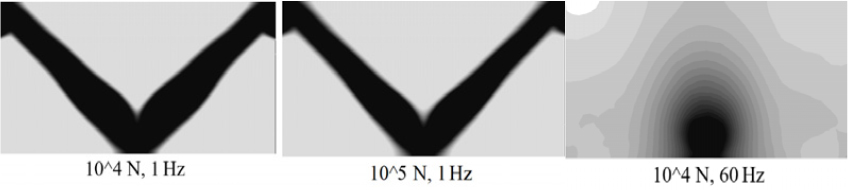
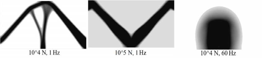
In case of rectangular model in Fig. 4, the first and second natural frequencies are 41.2 Hz and 76.1 Hz. In this example, 1 Hz lower than the first mode and 60 Hz higher than the first mode are used as excitation frequencies. It is generally known that when excitation frequency is lower than the first mode, a solution with an increased natural frequency is derived. When excited on 1 Hz, a stiffer shaped solution is derived, but the first natural frequency of solution is decreased to 13.8 Hz. This is expected to occur because the Young’s modulus of the loaded area is reduced by 90 %. In addition, the result is similar to the solution of thermal problem when excited at 1 Hz and 10⁴ N. However, when the loading is 10⁵ N, the result becomes similar to that of uniform temperature. Since it is a function in the frequency domain for the dynamical problem, it reflects only the Young’s modulus reduction without the static thermal load. Thus, the result is different from the case for thermoelastic problem. When the excitation frequency is 60 Hz, as in the paper of Olhoff and Du^[12] the first natural frequency is reduced close to rigid body motion and the result is disconnected from excitation area to the boundary.

As shown in Figs. 16 and 17, the results of calculating the various temperature distributions are derived differently from the thermoelastic problems. Likewise, it is expected that only Young’s modulus is reflected. And, in the case of this dynamic problem, if the number of meshes or modes is not large enough, it is difficult to obtain a symmetrical result from the design of numerical analysis. As the Young’s modulus is affected by the density model and the temperature distribution at the same time, it is expected that the solution is reflected more sensitively than the case of the density model.

https://cdn.apub.kr/journalsite/sites/ask/2026-045-02/N0660450205/images/ASK_45_02_05_F16.jpg

Fig. 16.

Effect of increased load forces using thermal case A and rectangular model in Fig. 4.

https://cdn.apub.kr/journalsite/sites/ask/2026-045-02/N0660450205/images/ASK_45_02_05_F17.jpg

Fig. 17.

Effect of increased load forces using thermal case B and rectangular model in Fig. 4.

3.1.3 Multi-objective problem

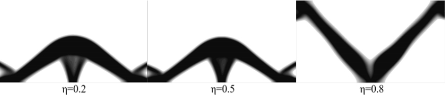
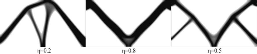
Multi-objective problem with rectangular model in Fig. 4 is performed using same material property of thermoelastic and dynamic problem. Optimization is performed for two heat distribution using 2 excitation frequency. 3 Weighting factors η (0.2, 0.5, 0.8) are used for analysis for each cases.

When the structure is excited at 1 Hz, the optimal solution for each temperature distribution is shown in Figs. 18 and 19. In the case of a solution applying the case B temperature distribution, when the weighting factor approaches 0 or 1, the pattern similar to the thermoelastic or dynamic solution is well seen, respectively. In the case of case A, similar trends using case B are shown. However, in case A, the η corresponding to the equilibrium point is expected to be slightly larger than 0.5. In the case of the current multi objective problem, this trend is observed because the same static and dynamic loading forces are used, but in reality, the static and the dynamic loading cannot be same. In addition, even when actual static and dynamic loads are applied, only one target of performance is serious for design. Therefore, it is necessary for the user to consider the appropriate force loading.

https://cdn.apub.kr/journalsite/sites/ask/2026-045-02/N0660450205/images/ASK_45_02_05_F18.jpg

Fig. 18.

Result of 1 Hz excitation on thermal load case A.

https://cdn.apub.kr/journalsite/sites/ask/2026-045-02/N0660450205/images/ASK_45_02_05_F19.jpg

Fig. 19.

Result of 1 Hz excitation on thermal load case B.

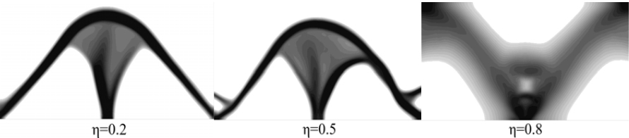
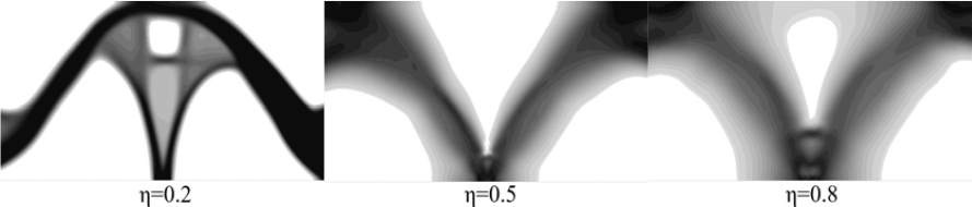
In the case of Figs. 20 and 21, it is the case that the dynamic problem and the thermoelastic problem, from which the unconnected solution is derived, are used as multi objectives. Because of the solution of thermoelastic problem of the connected shape, there is an advantage that the solution of the connected form is obtained. However, there is a limitation in that many gray scale elements are found.

https://cdn.apub.kr/journalsite/sites/ask/2026-045-02/N0660450205/images/ASK_45_02_05_F20.jpg

Fig. 20.

Result of 60 Hz excitation on thermal load case A.

https://cdn.apub.kr/journalsite/sites/ask/2026-045-02/N0660450205/images/ASK_45_02_05_F21.jpg

Fig. 21.

Result of 60 Hz excitation on thermal load case B.

The compliance values are compared in Tables 4 and 5 uisng Case A and different excitation frequencies. When the η (thermal load) is large, compliance is largely reduced after optimization. However, the compliance values of the optimal solutions are similar even in different excitation frequencies. Although similar compliance values are obtained under different excitation frequencies, the underlying mechanism cannot be clearly identified based on the present results alone.

Table 4.

Compliance comparison of 1 Hz excitation on thermal load case A.

η	0.2	0.5	0.8
Compliance initial	0.255	0.637	1.020
Compliance after	0.221	0.164	0.079

Table 5.

Compliance comparison of 60 Hz excitation on thermal load case A.

η	0.2	0.5	0.8
Compliance initial	0.142	0.355	1.256
Compliance after	0.101	0.144	0.111

3.2 A Vane of heat pump model

A vane model to control air stream of heater is chosen as a sample problem. In extremely cold condition, electric heater is often used to fulfill the necessary capacity. When electric heater is used for heating, the inlet air temperature on a vane can be higher than 100 °C and outlet air temperature is around 40 °C to prevent injury by heat. The problem is that shape of vane is generally long and slender, therefore it can be largely deformed in this heating condition. In addition, the material of vane is generally chosen for product appearance design with polymers. Therefore the materials with temperature dependent Young’s modulus are frequently applied for vane.

A long and slender vane model of indoor is shown as Fig. 22. The material properties are defined close to that of Acrylonitrile Butadiene Styrene (ABS). Young’s modulus (E₀), Poisson ratio (ν), and heat expansion ratio (α) are 2.0 GPa, 94.5 × 10^–6/K and 0.3. The loaded force F, target volume fraction and thermal conductivity coefficient are 10⁶ N, 0.2 and 0.0008 W/mK. Heat expansion ratio is much larger than metal but thermal conductivity coefficient is much lower than metal. However, the dimensions, shapes of the vanes and temperature distribution are conveniently chosen for calculation with asymmetric boundary condition. 10 Hz and 170 Hz are used for excitation frequency.

https://cdn.apub.kr/journalsite/sites/ask/2026-045-02/N0660450205/images/ASK_45_02_05_F22.jpg

Fig. 22.

A Vane of heat pump model and temperature distribution (Thermal loading).

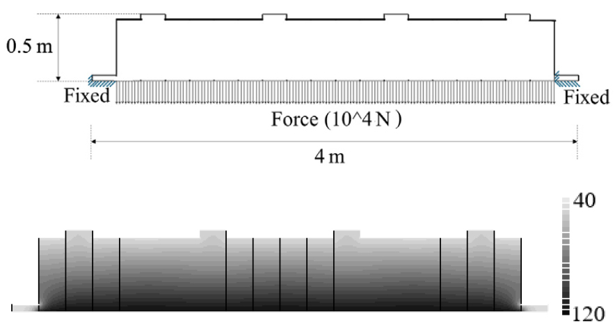
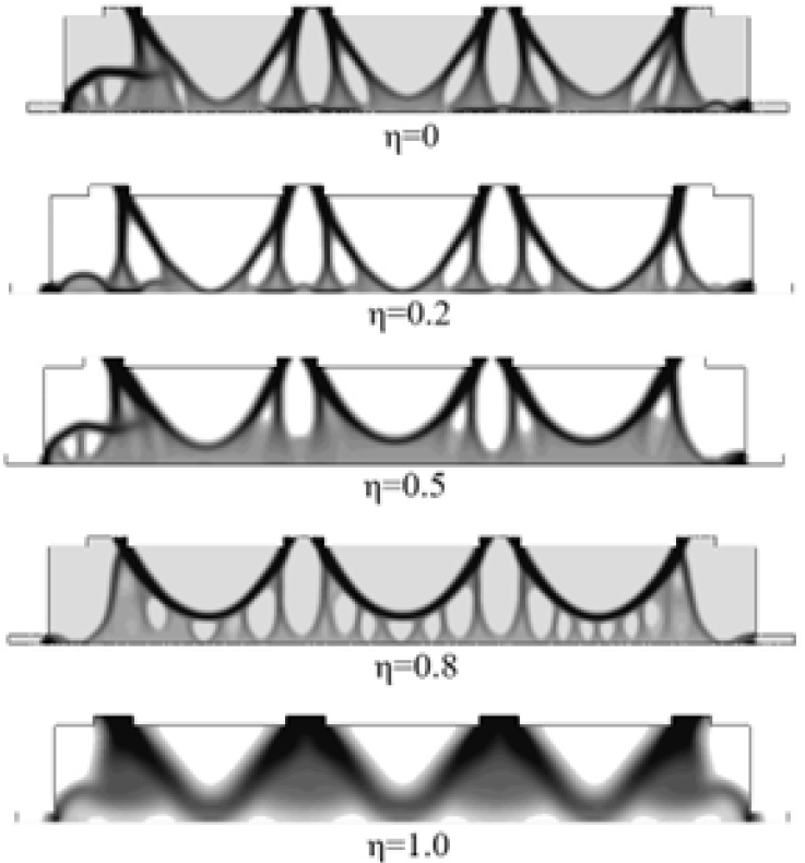
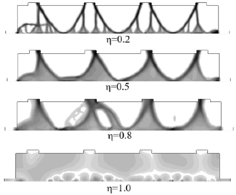
The minimum and maximum temperature of the model are 40 °C and 120 °C. The simplified temperature dependent Young modulus are given as Fig. 23. The optimization results using 2 excitation forces are shown in Figs. 24 and 26. The temperature distributions after calculation are similar to each other, representative of which is shown in Fig. 25. The trend of result is that elements of higher density is used in low temperature area to reduce heat expansion but arch of bridge type structure are generated to reduce harmonic response. In the case of a solution in which only a dynamic problem is considered for complex model, many gray scale elements have been derived, and the mode superposition method is used, so it is very difficult to obtain a solution with a clear boundary due to the lack of modes. However, this example is quite close to real application case. When 10 Hz and 170 Hz are used for excitation and η is small, it looks very reasonable solution to apply component design.

https://cdn.apub.kr/journalsite/sites/ask/2026-045-02/N0660450205/images/ASK_45_02_05_F23.jpg

Fig. 23.

Temperature dependent Young’s modulus of a vane model.

https://cdn.apub.kr/journalsite/sites/ask/2026-045-02/N0660450205/images/ASK_45_02_05_F24.jpg

Fig. 24.

Result of 10 Hz excitation and thermal load.

https://cdn.apub.kr/journalsite/sites/ask/2026-045-02/N0660450205/images/ASK_45_02_05_F25.jpg

Fig. 25.

Updated temperature distribution of 10 Hz and thermal load.

https://cdn.apub.kr/journalsite/sites/ask/2026-045-02/N0660450205/images/ASK_45_02_05_F26.jpg

Fig. 26.

Result of 170 Hz excitation and thermal load.

IV. Conclusion

This paper proposed a structural topology optimization method of thermoelastic problem considering temperature dependent Young’s modulus. Simple linear model is suggested and example problem are solved to show the influence of this model. The achievement of this research can be concluded as follows:

(a) A linear temperature dependent Young’s modulus model is suggested considering amorphous thermoplastic polymer.

(b) In the thermoelastic problem, the application of temperature-dependent Young’s modulus model changes the balance of structural and thermal stresses, resulting in a new shape solution.

(c) In the dynamic problem, as the Young’s modulus changed, a solution with a different shape from constant Young’s modulus were derived. The solution in which the excitation point and boundary are not connected according to the relationship between the excitation frequency and the natural frequency is similar to former research.

(d) When multi objective problems are applied, connected solutions can be derived even if the solution of the dynamic compliance minimization problem is not connected from excitation point to the boundary.

(e) Thermoelastic and vibration problems are known to cause frequent gray scale elements. Most of calculation time is used to remove gray scale elements. Adaptive mesh has the advantage of clarifying the boundaries where gray scale elements occur mainly, it’s good to save computational cost.

Therefore, the results of this study are expected to be a good reference for actual design.

References

C. Lee, B. Kang, B.-H. Choi, J. Lee, and K. Lee, “Observation and characterization of squeak noises of polymeric materials for automotive interior parts under field-degradation,” Trans. KSAE, 25, 257-265 (2017).

10.7467/KSAE.2017.25.2.257

J. A. O. Bruno, N. L. Allan, T. H. K. Barron, and A. D. Turner, “Thermal expansion of polymers: Mechanisms in orthorhombic polyethylene,” Phys. Rev. B, 58, 8416-8427 (1998)

10.1103/PhysRevB.58.8416

H. Rodrigues and P. Fernandes, “A material based model for topology optimization of thermoelastic structures,” Int. J. Numer. Methods Eng. 38, 1951-1965 (1995).

10.1002/nme.1620381202

Q. Li, G. P. Steven, and Y. M. Xie, “Thermoelastic topology optimization for problems with varying temperature fields,” J. Therm. Stresses, 24, 347-366 (2001).

10.1080/01495730151078153

Q. Xia and M. Y. Wang, “Topology optimization of thermoelastic structures using level set method,” Comput. Mech. 42, 837-857 (2008).

10.1007/s00466-008-0287-x

T. Gao and W. Zhang, “Topology optimization involving thermo-elastic stress loads,” Struct. Multidisc. Optim. 42, 725-738 (2010).

10.1007/s00158-010-0527-5

H. Chung, O. Amirb, and H. A. Kima, “Level-set topology optimization considering nonlinear thermoelasticity,” Comput. Meth. Appl. Mach. Eng. 361, 1-50 (2020).

10.1016/j.cma.2019.112735

J. Zheng, X. Rong, and C. Jiang, “Thermoelastic topology optimization for structures with temperature-dependent material properties,” Sci. China Technolo. Sci. 66, 3488-3503 (2023).

10.1007/s11431-023-2458-6

Y. Chen, L. Ye, Y. X. Zhang, and C. Yang, “A multi material topology optimization with temperature dependent thermoelastic properties,” Eng. Optim. 54, 2140-2155 (2022).

10.1080/0305215X.2021.1977291

Z.-D. Ma, N. Kikuchi, and I. Hagiwara, “Structural topology and shape optimization for a frequency response problem,” Comput. Mech. 13, 157-174 (1993).

10.1007/BF00370133

S. Min, N. Kikichi, Y. C. Park, S. Kim, and S. Chang, “Optimal topology design of structures under dynamic loads,” Struct. Multidisc. Optim. 17, 208-218 (1999).

10.1007/BF01195945

N. Olhoff and J. Du, “Generalized incremental frequency method for topological design of continuum structures for minimum dynamic compliance subject to forced vibration at a prescribed low or high value of the excitation frequency,” Struct. Multidisc. Optim. 54, 1113-1141 (2016).

10.1007/s00158-016-1574-3

L. Shu, M. Y. Wang, Z. Fang, Z. Ma, and P. Wei, “Level set based structural topology optimization for minimizing frequency response,” J. Sound. Vib. 330, 5820-5834 (2011).

10.1016/j.jsv.2011.07.026

O. M. Silva, M. M. Neves, and A. Lenzi, “A critical analysis of using the dynamic compliance as objective function in topology optimization of one-material structures considering steady-state forced vibration problems,” J. Sound Vib. 444, 1-20 (2019).

10.1016/j.jsv.2018.12.030

I. M. Ward and J. Sweeney, Mechanical Properties of Solid Polymers, 3^rd Ed (A John Wiley and Sons, Ltd. Chichester, 2013), pp. 135-166.

M. Nasraoui, P. Forquin, L. Siad, and A. Rusinek, “Influence of strain rate, temperature and adiabatic heating on the mechanical behavior of poly-methyl-methacrylate: Experimental and modelling analyses,” Mater. Des. 37, 500-509 (2012).

10.1016/j.matdes.2011.11.032

I. H. Sahputra, A. Alexiadis, and M. J. Adams, “Temperature dependence of the Young’s modulus of polymers calculated using a hybrid molecular mechanics–molecular dynamics method,” J. Phys. Condens. Matter. 30, 1-19 (2018).

10.1088/1361-648X/aad588

G. Allaire, Numerical Analysis and Optimization (Oxford University Press, New York, 2009), pp. 1-28.

C. Kim, M. Jung, T. Yamada, S. Nishiwaki, and J. Yoo, “FreeFEM++ code for reaction-diffusion equation-based topology optimization: for high-resolution boundary representation using adaptive mesh refinement,” Struct. Multidisc. Optim. 62, 439-455 (2020).

10.1007/s00158-020-02498-3

T. Yamada, K. Izui, S. Nishiwaki, and A. Takezawa “A topology optimization method based on the level set method incorporating a fictitious energy,” Comput. Meth. Appl. Mech. Eng. 199, 2876-2891 (2010).

10.1016/j.cma.2010.05.013

H. Li, T. Yamada, P. Jolivet, K. Furuta, T. Kondoh, K. Izui, and S. Nishiwaki, “Full-scale 3D structural topology optimization using adaptive mesh refinement based on the level-set method,” Finite Elem. Anal. Des. 194, 276-308 (2021).

10.1016/j.finel.2021.103561

The Journal of the Acoustical Society of KoreaISSN:1225-4428(Print) 2287-3775(Online)한국음향학회