I. Introduction

There are many diverse areas in system applications of fiber optic sensors.^[1-5] Fiber optic interferometric sensor has many significant advantages and in many applications several of the advantages can apply.^[6,7] Some of the advantages are increased sensitivity, EMI (Electro-Magnetic Interference) immunity, large bandwidth, and geometrical versatility.^[4,5] To detect external sound signals using the compliant hollow mandrel which wrapped by optical fiber, Sagnac interferometer can be fabricated and tested.^[7-9] The effect of an acoustic field acting on a coil is causing a change in the optical path length of the coil, and this can be detected as a phase change in light passing through the coil.^[8] Compliant hollow cylindrical mandrel has been widely used to make fiber optic acoustic sensors.^[7-9]

The principle of the Sagnac interferometer is consist of input light split into two parts at the 2 × 2 coupler (beam splitter) and the two lights rotate in an opposite direction to each other, then come together in 2 × 2 coupler.^[1,2] Photo diode detected the output signal with information of physical variation which experienced in the loop. Phase differences between the two lights are directly proportional to the acoustic and vibration pressure in the loop. Detected signal intensity is also proportional to the phase difference. The two lights rotate the loop and phase difference is expressed as^[3]

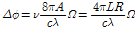, (1)

where R is the radius of closed loop, is the angular velocity, v is the tangential velocity, λ is the wavelength, c is the speed of the light, and L is the total loop length.

In Eq.(1), the sensitivity or phase difference of the fiber optic sensor in Sagnac interferometer is proportional to the closed loop length (L). Sagnac interferometer with fiber optic sensor can be used as a diagnostic system of the electrical power equipment. Degradation and partial discharge are common causes of electrical power transformer system. General diagnostic sensor used in the electrical power system has weak point such as large scale and long measurement time.

Using Sagnac interferometer, previous research presented sound pressure detection with single sensor element. Therefore, the purpose of this research is to detect the two different acoustic signals generated in the cylindrical cavity submerged in transformer oil by using fiber optic sensor array in one Sagnac loop. Because of space limita-tions in the cylindrical cavity, two sensors were fabricated in one loop.

This paper is organized in the following arrangements. Section II provides an experimental setup and shows fiber optic sensor array in the transformer oil. Section III presented the experimental results and discussion, and finally the concluding remarks are summarized in Section IV.

II. Experimental Setup

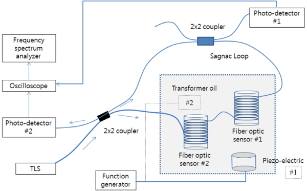
Experimental setup using Sagnac interferometer with two fiber optic sensors in the loop is shown in Fig. 1. Photograph of the experimental setup is shown in Fig. 2. TLS (Tunable Laser Source) supplied light to the Sagnac loop and two photo-detectors were used.

Two fiber optic sensors connected in serial were used while being submerged into transformer oil. Outside sound pressure was directly applied to the sensors using piezoelectric generator which wound optical fiber. The two sound sources were generated by function generator which controlled under different frequencies.

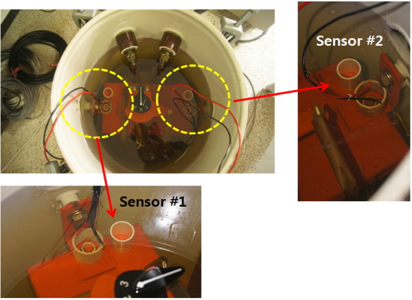
Generally, the performance of fiber optic acoustic, electric and magnetic field sensors are known. The fiber wrapped on a compliant hollow mandrel yields highest sensitivity.^[8] Therefore, in this experiment, optical fiber's total length of 48.6 m was wrapped on a CRP (Carbon Reinforced Plastic) hollow mandrel, as shown in Fig. 2. The distance between two sensors is 30 cm and length of the Sagnac loop is 1.7 m. Photograph of the two fiber optic acoustic sensors and sound generator are also shown in Fig. 2.

Physical quantities of the transformer oil such as viscosity, specific weight, and sound speed are 8.5 cSt., 0.86, and 1,095 m/sec, respectively. The distance between sound generator and sensor is 10 cm each. Experiments were continued by changing applied sound frequency from 5 kHz to 90 kHz. The wavelength of the 35 kHz sound is 2.86 cm in the transformer oil.

This is a first attempt to analyze the sound frequency using two fiber optic sensors in one Sagnac loop. Because there are many electrical parts in the cylindrical transformer (described in Fig. 2), fiber optic sensors have limited space.

III. Experimental Results and Discussion

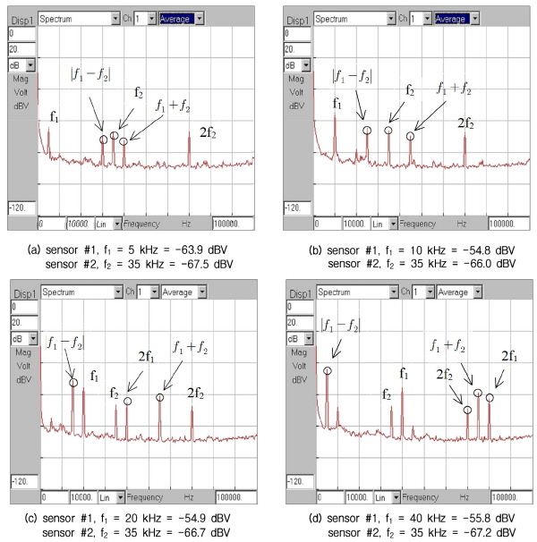
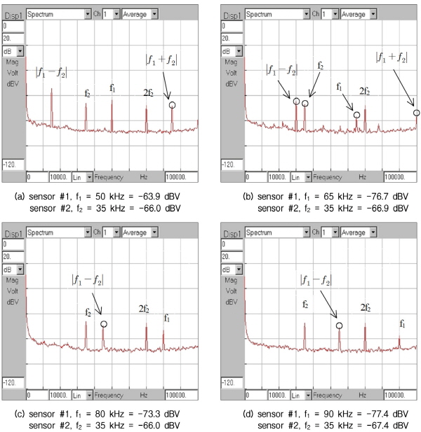
Applied sound frequency was fixed at = 35 kHz in the fiber optic sensor #2. Under that condition, fiber optic sensor #1 was continued by changing applied sound frequency from 5 kHz to 90 kHz. Figs. 3 and 4 show detected amplitude comparison in terms of arbitrary applied sound frequencies () such as 5, 10, 20, 40, 50, 65, 80, and up to 90 kHz. Most results contained harmonic frequencies of the applied sound frequency. These harmonic frequencies probably come from the shape of the circular container.

In Figs. 3 and 4, applied frequency and fixed frequency are and , respectively. From those figures, harmonic frequencies and overtones of and appeared mostly. In low frequency cases such as 5 kHz and 10 kHz of , harmonic frequency of was not observed because of their long wavelength distances (20 cm at 5 kHz compared to 10 cm at 10 kHz).

Those harmonic frequencies such as , , , were came from the shape of the container. It is known that the Sagnac interferometer is comparable to Mach-Zehnder interferometer when the signal frequency matches the length of the Sagnac loop.

The Helmholtz equation of the right circular cylindrical cavity with height (L) and radius (a) shown in Fig. 2 is expressed as

, (2)

where , is circular frequency, and is wave number. In cylindrical coordinates , the Helmholtz equation, Eq.(2), becomes^[10]

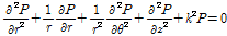, (3)

where is the pressure amplitude, . Using boun-dary conditions and separation of variables, the pressure of the mode is expressed as^[10]

, (4)

where , is th Bessel function of the first kind, and are constant numbers. The angular frequencies are determined from^[10]

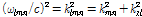, (5)

where c is the wave speed. From Eqs. (4) and (5) it is clear that the pressure of the certain mode is function of frequency.

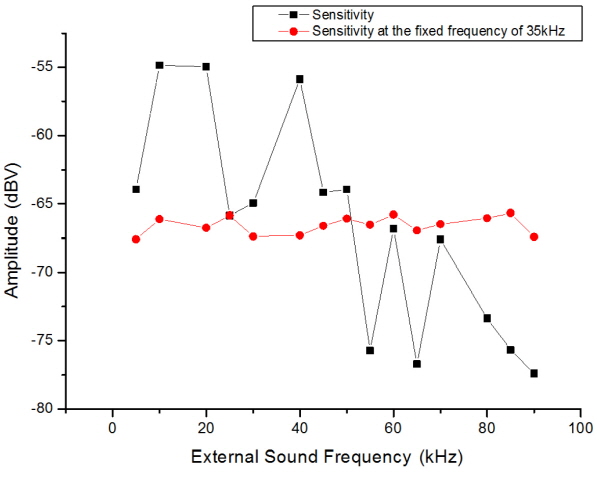
Detected amplitude comparison between applied sound frequency and fixed frequency is shown in Table 1 and Fig. 5. At frequency under 50 kHz, amplitude is greater than the case of fixed frequency shown in Fig. 3 (a) to (d). However, frequency above 50 kHz amplitude is lower than the case of fixed frequency, as shown in Fig. 4 (a) to (d).

From this experiment it is confirmed that fiber optic sensor using Sagnac interferometer in the transformer oil can detect harmonic series of applied sound frequency such as , , , .

Because of sensor dimension (mandrel diameter and height) this experimental approach is limited to certain space. However, in real electric transformer system, suggested fiber optic sensor array can be applied to monitor physical quantities such as internal temperature, sound pressure, vibration due to partial discharge, etc. In addition, other application can be expanded to the underwater sonar system.

IV. Conclusions

This paper attempted to confirm overtones and harmonic series in the cylindrical cavity which put in transformer oil using fiber optic Sagnac loop. Optical fiber's total length of 48.6 m was wrapped surrounding the compliant hollow mandrel (CRP) as an optical fiber sensor. Two different external sound frequencies, and , were applied to the sensor array simultaneously by using piezoelectric with frequency range from 5 kHz to 90 kHz. Based on the experimental results fiber optic sensor detected overtones and harmonic series of applied sound frequency such as , , , , , . Below 50 kHz of applied sound frequency, the sensitivity is higher than the fixed case, while above 50 kHz, the results are lower than the fixed case. In real electric transformer system, suggested fiber optic sensor array can be applied to monitor physical quantities such as internal temperature, sound pressure, and vibration due to partial discharge.