I. Introduction

The gold standard methods for the assessment of osteoporosis and bone status are based on Dual Energy X-ray Absorptiometry (DEXA) or, to be more precise, on a two-dimensional or three-dimensional image mapping of the X-ray absorption coefficient, which can then be translated into a Bone Mineral Density (BMD) image.^[1] Although the BMD is an important predictor of the bone strength, additional parameters including tissue-intrinsic material properties and bone architecture are required to explain the bone strength more accurately.^[2] However, X-ray based absorptiometry techniques can only provide limited information on the mineralization and the geometry of bones in two-dimensional projection mode. In addition, they have some other disadvantages, such as the presence of ionizing radiation, poor portability, and relatively high cost.

In order to overcome these limitations, Quantitative UltraSound (QUS) is now widely used as an attractive alternative to DEXA. Most of the current bone sonometers measure the speed of sound and/or the broadband ultrasound attenuation at easily accessible peripheral sites mostly consisting of trabecular bone (typically the calcaneus).^[3] One of the limitations of QUS techniques in clinical practice is their restricted application to the peripheral skeletal sites only instead of the fracture sites. Human long bones such as the femur, the radius, and the tibia have a thick outer layer of cortical bone. The thickness of the cortical layer has been shown to correlate significantly with the fracture load at the radius, the femur, and the lumbar vertebrae.^[4] The cortical bone thickness can be determined with X-ray based absorptiometry techniques that use ionizing radiation, at peripheral sites such as the radius and the tibia. However, a cheap, simple, radiation-free, and accurate method for multi-site determination of the cortical bone thickness is clinically desirable.

The present study aims to investigate the feasibility of two different ultrasonic methods for measuring the cortical bone thickness in bovine tibia in vitro. In the reflection technique, the tibial cortical thickness was determined from ultrasonic reflections from the periosteum and the endosteum producing specific peaks in the signal envelope. In the axial transmission technique, the tibial cortical thickness was determined from ultrasonic guided wave velocities measured along the axial direction of the tibia. The performance of the reflection and the axial transmission techniques in determining the cortical bone thickness was compared.

II. Materials and methods

Twenty eight fresh bovine tibiae were acquired from a local slaughterhouse. Their proximal ends were removed by using a rotary electric saw to make a hollow tube- shaped tibia without any soft tissue and marrow. All the tibiae were defatted by water jetting and kept frozen at –20 °C before ultrasonic measurements. Ultrasonic measurements were performed at the tibial mid-shaft with a least irregularly shaped area, where the cortical thickness was relatively well defined. Fig. 1 shows a cross-sectional image of the tibial mid-shaft. The gray rectangular area indicates a region of interest interrogated with ultrasound within which the cortical bone thickness was determined. For each tibia, the mean thickness of the cortical layer was determined at ten different sites along the axial direction of the tibia by using a caliper with 0.05-mm resolution. The tibial mid-shaft was covered by a 2 mm-thick silicone rubber layer that simulates the soft tissue surrounding the cortical shell of long bones. The silicone rubber has an attenuation coefficient of about 1 dB/cm at 1 MHz and a longitudinal velocity of 1230 m/s.^[5] The attenuation coefficient of silicone rubber is very similar to that of muscle (1.09 dB/cm/MHz).^[6]

Fig. 1.

Cross-sectional image of the tibial mid-shaft. The gray rectangular area indicates a region of interest interrogated with ultrasound within which the cortical bone thickness was determined.

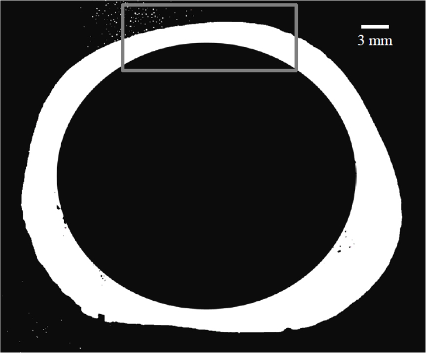
Fig. 2 shows a schematic diagram of the experimental setup for ultrasonic measurements by using the reflection technique with a transducer with a center frequency of 2.25 MHz and a diameter of 12.7 mm (V306, Panametrics, Waltham, MA). The transducer (as a transmitter and a receiver) was positioned perpendicularly to the periosteal boundary of cortical layer. An ultrasonic gel was applied for acoustic coupling between the transducer and the silicone rubber layer. The transducer was excited by using a pulser/receiver (5800PR, Panametrics, Waltham, MA). The Radio-Frequency (RF) signals were digitized by using a digital storage oscilloscope (WS44Xs, LeCroy, Chestnut Ridge, NY) averaging over 100 waveforms and then stored on a personal computer for off-line analysis.

Fig. 2.

Schematic diagram of the experimental setup for ultrasonic measurements by using the reflection technique with a transducer with a center frequency of 2.25 MHz and a diameter of 12.7 mm.

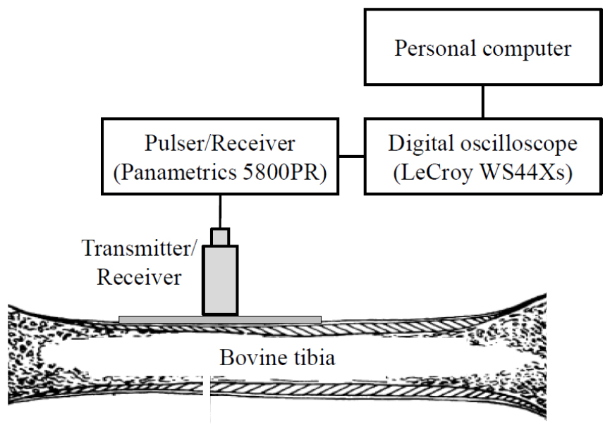
Fig. 3 shows the procedure for calculating the time difference. As seen in the RF signal, reflections from the periosteum and the endosteum can be observed. The envelope was calculated as a magnitude of the discrete- time analytic signal obtained by using the Hilbert transformation. The cortical bone thickness of the tibia, CTh_REF, was determined by using

where c is the radial longitudinal wave velocity of 4000 m/s in cortical bone^[7] and Δt is the time difference of the two maxima in the envelope. The cortical thickness was determined at ten different sites for each tibia. The thinnest cortical thickness measured by using a caliper in the present study was 1.95 mm. The minimum cortical thickness detectable with the reflection technique was 1.16 mm, which was determined from the pulse width of the 2.25-MHz transducer (5.58 μs) and the radial longitudinal wave velocity in cortical bone (4000 m/s).

Fig. 3.

(a) RF signal for reflections from the periosteum and the endosteum and (b) envelope calculated as a magnitude of the discrete-time analytic signal obtained by using the Hilbert transformation.

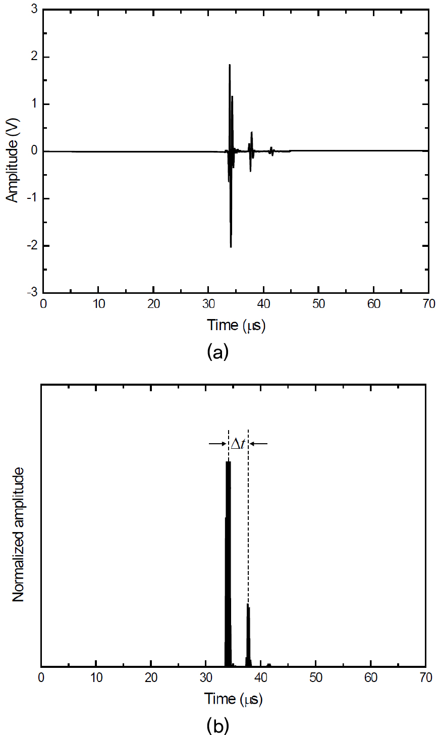
Fig. 4 shows a schematic diagram of the experimental setup for ultrasonic measurements by using the axial transmission technique with a pair of custom-made transducers with a center frequency of 200 kHz and a diameter of 12.7 mm. The distance between the transmitter and the receiver increased from 30 mm to 60 mm in 0.5-mm steps, which was measured from the center of the transducers. The receiver was horizontally moved along the long axis of the tibia under computer control. Each tibia was measured ten times.

Fig. 4.

Schematic diagram of the experimental setup for ultrasonic measurements by using the axial transmission technique with a pair of custom-made transducers with a center frequency of 200 kHz and a diameter of 12.7 mm.

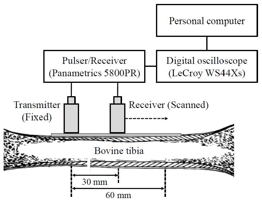
Fig. 5 shows the procedure for calculating the ultrasonic guided wave velocities. As seen in the RF signal, the shape of the RF signal exhibits the presence of at least two distinct propagating waves with different velocities, the fast First Arriving Signal (FAS) and the energetic Slow Guided Wave (SGW).^[8] The FAS and the SGW were consistently observed in all the tibiae. In order to determine their phase velocities, the absolute amplitude of the RF signal recorded at each transmitter-receiver distance was converted into gray level with the maximum amplitude corresponding to white and plotted as a horizontal line. As seen in Fig. 5(b), these horizontal lines were vertically stacked to give a diagram for visualizing propagating waves and for fitting a line to peaks within a wave packet. Tracking of the FAS was performed by using the earliest detectable deviation from zero because its amplitude was generally low. The SGW was tracked by using the peak maximum within the slower wave packet. Then, the phase velocities of the FAS and the SGW were determined as the slopes of the linear regression fits to the points in each wave packet. They have shown to be essentially consistent with the phase velocities of the fundamental symmetric (S0) and the antisymmetric (A0) Lamb waves propagating in a free cortical bone plate, respectively, when the cortical thickness is less than the wavelength.^[9]

Fig. 5.

(a) RF signal recorded at a transmitter-receiver distance of 60 mm and (b) absolute amplitude of the RF signal as functions of time (horizontal axis) and transmitter-receiver distance (vertical axis).

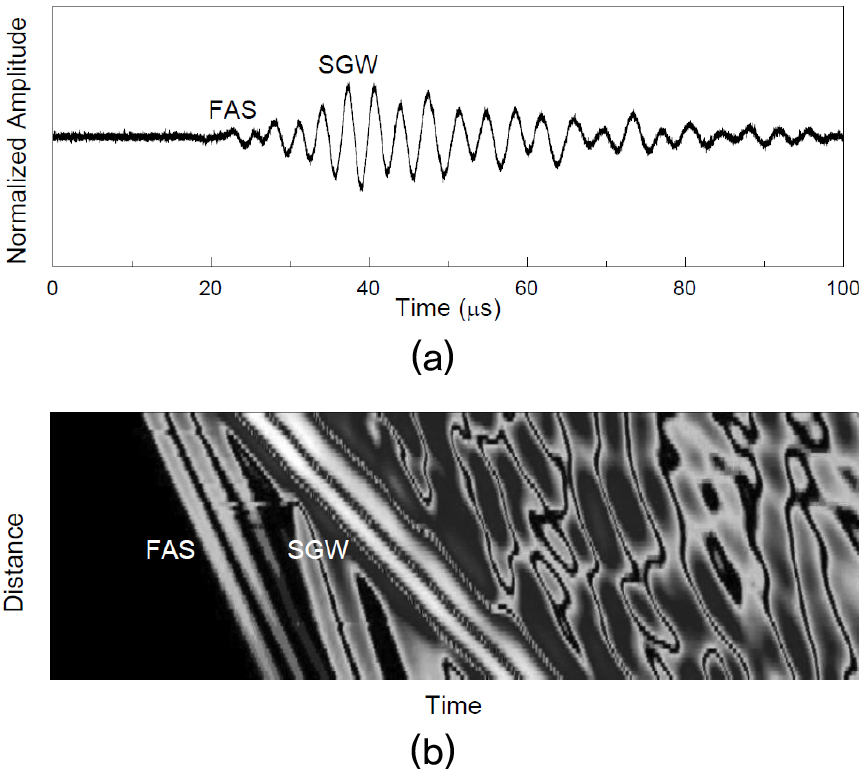
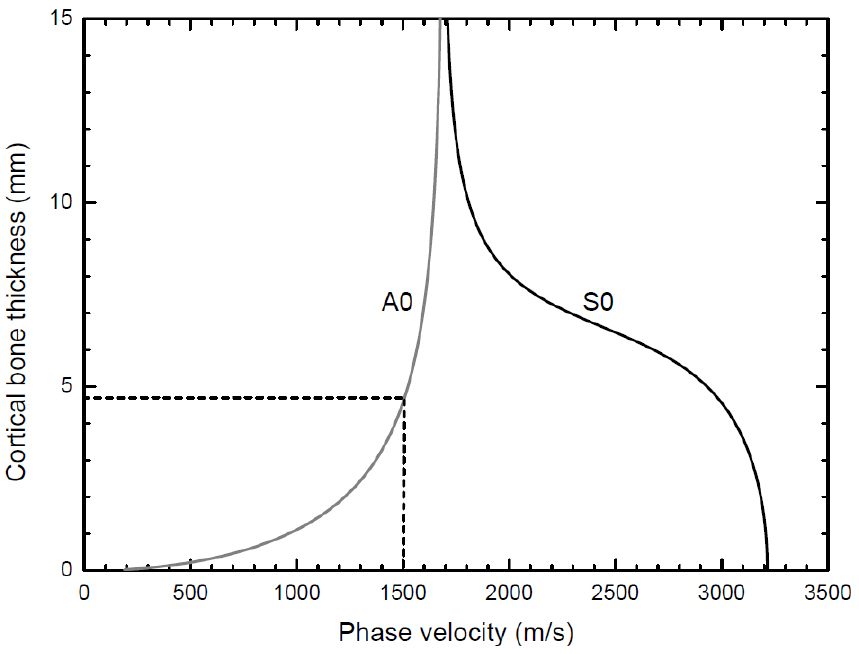
Fig. 6 shows the phase velocity dispersion curves of the 200-kHz S0 and the A0 Lamb waves predicted by using the Lamb wave theory for elastic wave propagation in a free solid plate, with the longitudinal and the shear wave velocities of 4000 m/s and 1800 m/s in cortical bone.^[7,10] The cortical bone thicknesses of the tibia, CTh_FAS and CTh_SGW, were determined from these dispersion curves. For instance, the SGW velocity (A0 Lamb wave velocity) of 1500 m/s corresponds to the CTh_SGW of about 4.8 mm.

Fig. 6.

Phase velocity dispersion curves of the 200- kHz S0 and the A0 Lamb waves predicted by using the Lamb wave theory with the longitudinal and the shear wave velocities of 4000 m/s and 1800 m/s in cortical bone.

III. Results and discussion

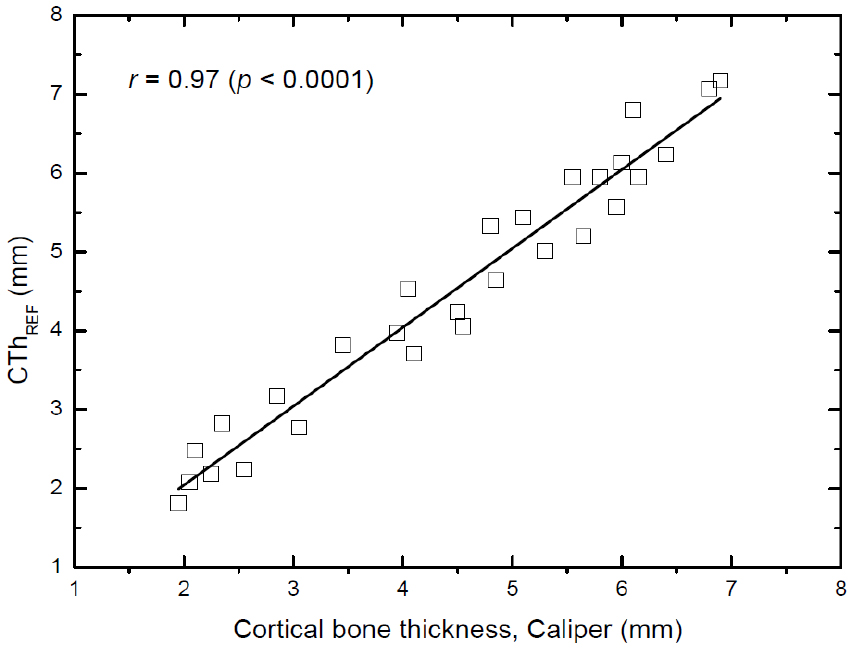
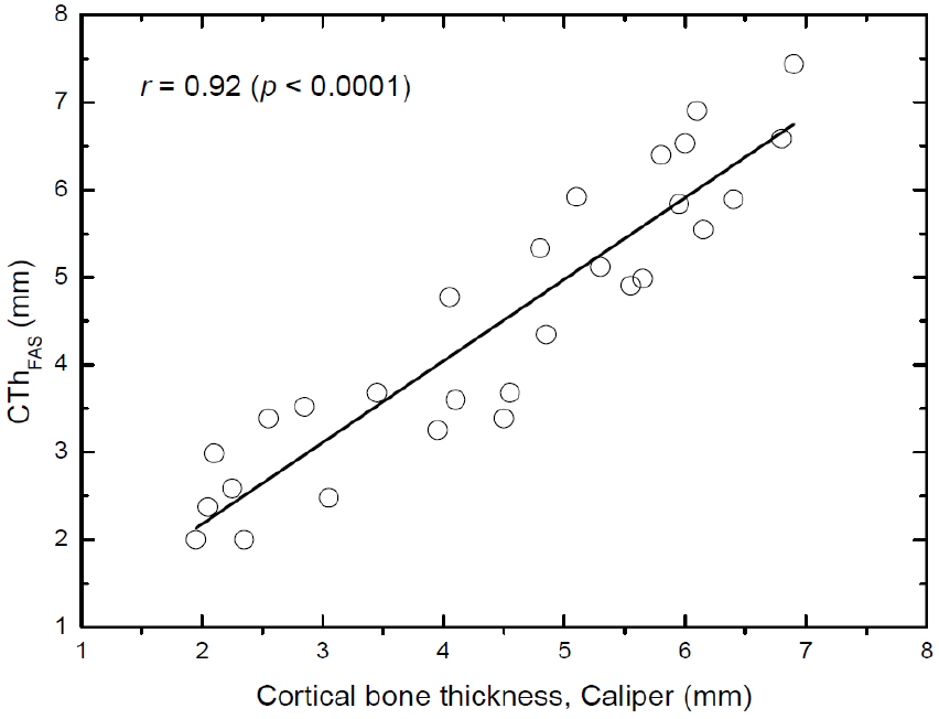
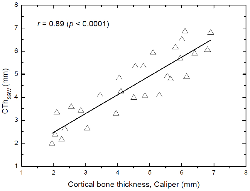
Figs. 7, 8, and 9 show the correlations of the cortical bone thickness determined by using the ultrasonic methods with that measured by using a caliper in the 28 bovine tibiae. Linear fits were performed between pairs of measurements to obtain Pearson’s correlation coefficients (r). As found in Fig. 7, the cortical bone thickness determined by using the reflection technique (CTh_REF) correlated significantly with that measured by using a caliper, with a correlation coefficient of r = 0.97 (p < 0.0001). The precision of the reflection technique measurements (mean value of the standard deviations of the measurements) was 0.22 mm. In contrast, the correlation coefficients for the axial transmission technique were r = 0.92 (p < 0.0001) for the CTh_FAS and r = 0.89 (p < 0.0001) for the CTh_SGW. The corresponding precisions were 0.39 mm for the CTh_FAS and 0.42 mm for the CTh_SGW.

Fig. 7.

Correlation of the cortical bone thickness determined by using the reflection technique (CTh_REF) with that measured by using a caliper in the 28 bovine tibiae.

Fig. 8.

Correlation of the cortical bone thickness determined by using the FAS method (CTh_FAS) with that measured by using a caliper in the 28 bovine tibiae.

Fig. 9.

Correlation of the cortical bone thickness determined by using the SGW method (CTh_SGW) with that measured by using a caliper in the 28 bovine tibiae.

In the present study, the in vitro feasibility and precision of the reflection and the axial transmission techniques for measuring the cortical bone thickness was investigated in the 28 bovine tibiae covered by a 2 mm-thick silicone rubber layer. The significant correlations between the cortical bone thickness measured by using the reflection technique and that measured by using a caliper seemed to be consistent with those previously reported in human tibia in vitro.^[11,12] For instance, Wear obtained high correlations between the estimated and the true cortical thickness with correlation coefficients of r = 0.92 for the autocorrelation method and r = 0.85 for the cepstral method in 6 human tibiae in vitro.^[11] The method presented in that study entails estimation of tibial cortical thickness by measurement of autocorrelation functions and cepstra of ultrasonic echoes from the tibial cortex. Although those techniques were found to be successful in determining the cortical bone thickness of human tibia in vitro, it is evident that the simplicity of the envelope method used in this study makes it more attractive for clinical applications.

The cortical bone thickness measured by using the axial transmission technique in the 28 bovine tibiae exhibited high but somewhat lower correlations with that measured by using a caliper compared to the reflection technique. These results is due to the fact that the phase velocities of the FAS and the SGW measured here are essentially consistent with those of the S0 and the A0 Lamb waves, respectively, when the cortical thickness is less than the wavelength.^[9] Assuming the longitudinal wave velocity of 4000 m/s in cortical bone, the wavelength is 20 mm at 200 kHz, less than the values of the cortical thickness (ranging from 1.95 mm to 6.90 mm) in the 28 bovine tibiae. The axial transmission technique used in the present in vitro study may have some limitations in predicting the cortical bone thickness in vivo. A challenge for clinical applications of the guided wave technique is the soft tissue layers overlying the cortical bone because guided waves are sensitive to conditions at waveguide boundaries. Moreover, the accuracy of the time-of-flight method applied in the technique may suffer from inaccuracy in determining the pulse arrival time due to the use of low frequencies.^[12] Hence, these sources of artifact warrants further attention. In spite of these difficulties, the use of the ultrasonic guided waves in bone is attractive because their velocities are strongly sensitive to the material properties throughout the entire thickness of cortical bone and thus captures pathological changes.^[9]

IV. Conclusions

The present study has validated the two different ultrasonic methods for measuring the cortical bone thickness in bovine tibia in vitro. The reflection technique was found to perform somewhat better on 28 bovine tibiae covered by a 2 mm-thick silicone rubber layer compared to the axial transmission technique. Human long bones have tubular structures with irregular shape, rough boundaries, and inhomogeneous, anisotropic elastic properties. Futhermore, they are filled by fat-like bone marrow and are surrounded by soft tissues of the human body. Clinical feasibility should be demonstrated with an in vivo application to address the question whether the ultrasonic methods presented here could be useful as a screening tool for osteoporosis and potentially could be applied to other skeletal sites such as the femur and the radius.