I. Introduction

Ocean surveillance systems generally employ highly sensitive passive sensors such as line arrays to localize underwater target of low frequency and long range. If the waves suffer horizontal refractions during their propagation, the passive sensors may fail to localize the underwater targets. The horizontal refractions can occur by the spatial variations of environment including bathymetry and sound speeds in water.

The simulation of horizontal refractions needs complete 3-Dimensional (3D) models rather than simple 2-Dimensional (2D) ones which manage only one directional wave fields between the source and receiver. Models based on the Parabolic Equation (PE) scheme are known to be efficient to compute the wave fields of low frequency.^[1] In simulating the horizontal refractions of acoustic fields, this study uses the 3D model, cuSPE0.9,^[2] developed by employing the parabolic equation scheme. The model is extended so that the RAnge-dependent Model (RAM)^[3,4] gives the 3D acoustic fields accepting environmental variations of bathymetry and sound speed profiles in water.

We briefly introduce the model schemes in section II, and show some simulation results focused on the horizontal refractions by the varying bathymetry in section III. Through the simulations, we can confirm the applicability of the model in simulating horizontal refractions of underwater acoustic waves. We also give a few issues of improvements to be operational in ocean surveillance systems.

II. Model implementation

2.1 Split-step padé algorithm

We employ the model developed based on the 3D parabolic equation algorithm including higher-order cross- terms.^[3] As a strategy to solve cross-terms, the algorithm splits the full exponential operator shown in previous works.^[5,6,7] We just give key expressions to arrive at solving cross-terms.

In the Cartesian coordinate (x,y,z), one-directional 3D energy-conserving PE for outgoing wave is given by^[5,8,9]

For the acoustic pressure p and reference wavenumber k_o,u=pe-jkox/α, where αis the energy-conserving parameter. The differential operators Y and Z are expressed by complex wavenumber, refractive index, density and sound speed.

When we assume the forward marching range x to be stair-step approximation, we can derive the split-step marching solution of Eq. (1) at range x+∆x as following

When we give Padé approximation to Eq. (2), we can have the full solution expressed by rational terms^[8]

Here ai and bi are Padé coefficients induced from rational terms. Eq. (3) requires a large number of numerical operations and leads to much computation time. One of the schemes of saving computation time is to separate operators Y and Z in the denominator. We employ the Chisholm approximation which converts 2D Taylor approximation into rational form as following

The coefficient in the nominator dij is induced from the Chisholm approximation. When we separate cross- and non cross-terms in terms of Y and Z in Eq. (2), we can get multiple form of the two kinds of terms.^[2] Applying Padé and Taylor approximations to non cross-terms and cross-terms respectively, we have the final expression to simulate 3D effects of environment with cross terms.

Here a^i and b^i are Taylor approximation coefficients. The Taylor approximation terms in ( ) represent cross-terms with the coefficient c_ij.

2.2 Parallelization

Eq. (5) still has multiples of rationals in terms of operators Y and Z, leading to sequential computation and keeping from parallel processing. If we give some modifications to the first two terms, we can have the form of summations which makes the independent parallel processing possible.

Here a^i and b^i are also approximation coefficients. In realizing the parallel processing, we employ three strategies:^[2] 1) parallelization of matrix inversion and multiplication with the first and second terms, 2) parallelization of matrix update, for example, the first term multiplied by temporary value of u(x), 3) parallelization of matrix inversion which uses the hybrid and parallel cyclic reduction algorithm provided in the CUDA sparse matrix library.^[10]

The simulation time depends on the numbers of matrix segment, block and thread where we find the optimum numbers as 60, 512 and 384, respectively.^[2] In an example with a Graphical Processing Unit (GPU, NVIDIA GTX- 1080) based PC (Intel i7-7700, 2 GPU) in an environment of wedge bathymetry and propagating range 16 km, we find about 22.7 min while 242.6 min of computation time with a CPU based PC (Intel i7-7700).^[2]

III. Simulations

3.1 Inputs

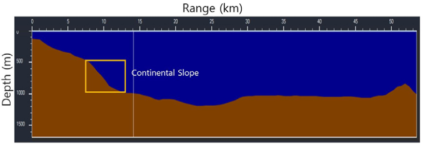
We present the simulation results of horizontal refractions of acoustic waves focusing on the bathymetry effects. The East Sea of Korea has bathymetry distributions of very big variations including continental shelf, slope and ridge. Specially, continental slope, a region of slope is about 4.3°,^[11] is very dominant. Fig. 1 shows an example of continental slope (box area).^[12]

Fig. 1.

(Color available online) An example of bathymetry section in the East Sea of Korea.

In simulating the horizontal refractions, we consider two kinds of bathymetry: 1) artificial distributions of ‘V’, inverse ‘V’, and wedge shapes, 2) real distributions from two different data sources.

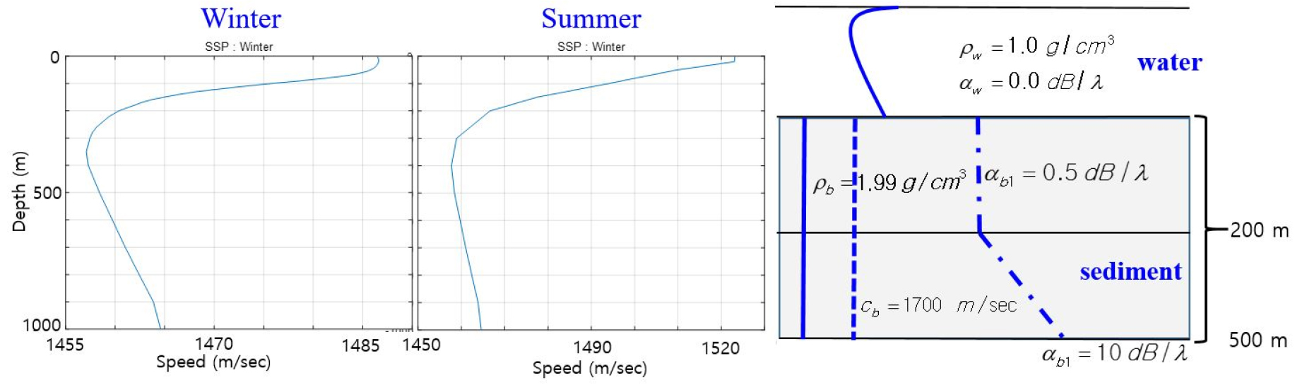
Concerning the input parameters to the model, we select typical profiles^[12] of winter and summer in water column, and typical geoacoustic properties in bottom sediment as shown in Fig. 2.

Fig. 2.

(Color available online) Input parameters to the model in the simulation region. (left & center) sound speed profiles in water column, (right) geoacoustic properties in bottom sediment.

The simulation assumes the Continuous Wave (CW) source of 75 Hz at depth 100 m (Zs) and cross range (Ys) 2 km, the area being 25 km (X, propagating) × 4 km (Y, crossing) in artificial bathymetry case.

3.2 Results

A. Artificial Bathymetry

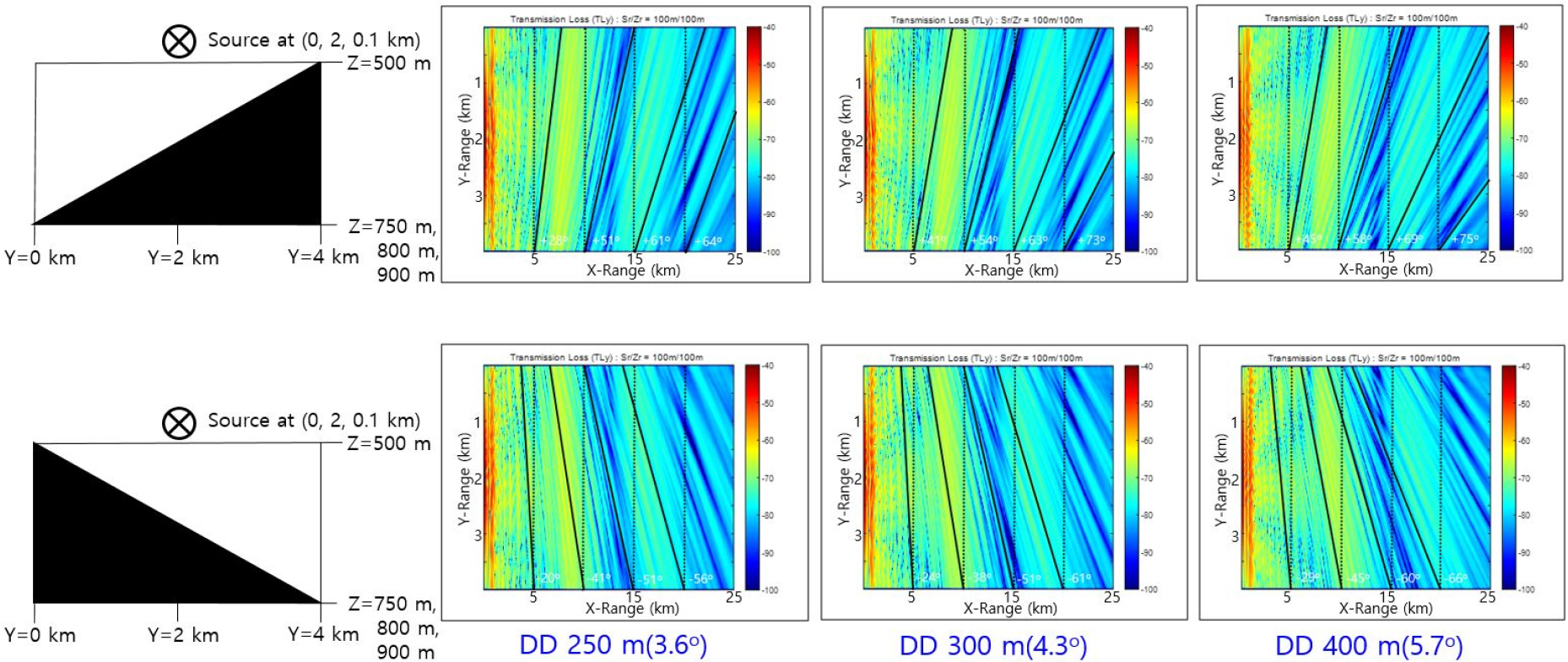
We try to check if the model properly responds to bathymetry changes. Fig. 3 gives the 1-st simulation results for inverse ‘V’ and ‘V’ shapes of bathymetry. The symbol ‘⊗’ denotes that sound source propagates into the paper at (Xs = 0 km, Ys = 2 km, Zs = 0.1 km) where bathymetry slope is 5.7°, varying between 700 m and 900 m. The two sets of result come from the simulation with winter (up) and summer (down) Sound Speed Profile (SSP), respectively. The transmission loss on the horizontal distribution (left) at Zr = 100 m presents perfect symmetric patterns in the upper and lower parts to the center, Ys = 2 km.

Fig. 3.

(Color available online) Simulation results for inverse ‘V’ shape (up) with winter SSP and ‘V’ shape (down) bathymetry with summer SSP for slopes +/- 5.7°.

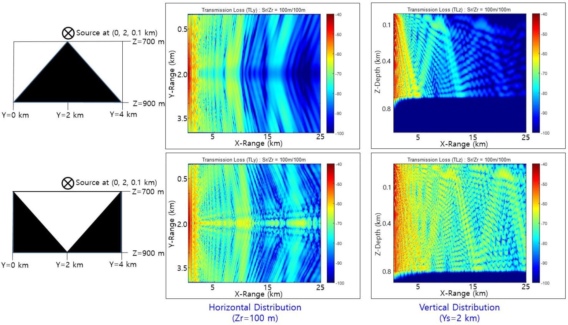
The transmission loss on the vertical distribution (right) at Xs = 0 km shows the convergence zone propagation structure. This structure is also clearly appeared on the transmission loss on the horizontal distribution (center) at the depth of 100 m, but the transmission loss patterns are curved depending on the bathymetry shape. We can say the sloping of convergence zones to be horizontal refraction caused by bathymetry distribution. The degree of the slope of transmission loss pattern shows nonlinear increase with propagating range, X.

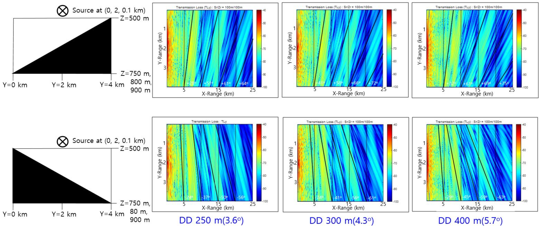
In order to examine the effect of sloping degree with the winter and summer SSP, we try other simulations with the wedge bathymetry. Fig. 4 shows the horizontal transmission loss with the bathymetry slopes 3.6°, 4.3°, and 5.7°. We make the slopes by changing the maximum depth from 750 m to 900 m, while the minimum depth is fixed at 500 m. We can see that the slope of the transmission loss pattern increases with the bottom slope increased. We use the winter SSP in the simulation. Another results with summer SSP (Fig. 5) give similar patterns of horizontal refraction to those with winter SSP.

Fig. 4.

(Color available online) Simulation results with wedge shaped bathymetry of variable slopes and winter SSP. ‘DD’ denotes the depth difference between the minimum and maximum.

Fig. 5.

(Color available online) Simulation results for wedge shaped bathymetry with variable slopes and summer SSP. ‘DD’ denotes the depth difference between the minimum and maximum.

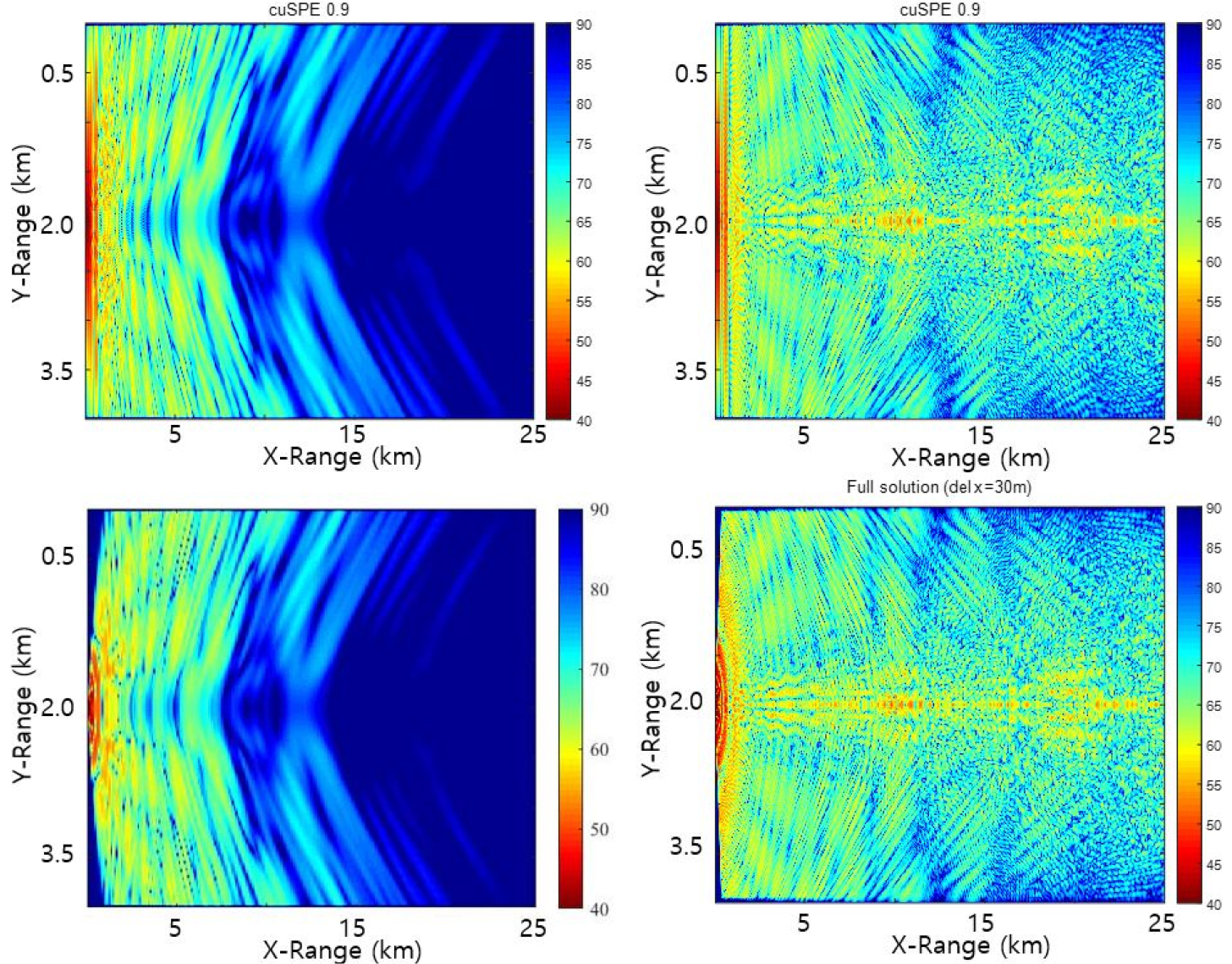
To compare the approximated solution of cuSPE0.9 with those of the full solution based on Eq. (3), we employ the simulation conditions of Fig. 3 but the bathymetry changes between 500 m and 900 m (slope is +/-11.3°). Fig. 6 gives the transmission loss distributions for inverse ‘V’ shape with winter SSP (left) and ‘V’ shape with summer SSP (right). The full solution comes from a MATLAB code and takes 55 h and 18 min while the cuSPE0.9 does about 5 h to get the results. Considerable portion of the time is estimated to be dedicated to creating transmission loss of crossing section (Y) at every propagating step (Y).

Fig. 6.

(Color available online) Simulation results comparison between the approximation [Eq. (6)] (up) and the full solution [Eq. (3)] (down) for bathymetry slopes +/- 11.3° of inverse ‘V’ shape with winter SSP and ‘V’ shape with summer SSP.

B. Real Bathymetry

To simulate the horizontal refractions in the real bathymetry, we use two kinds of bathymetry data, Korean Topography (KTOPO) and Earth Topography and Bathymetry (ETOPO1).^[12] The KTOPO has resolution up to 30 m × 30 m grid and covers the sea around Korean Peninsula, while the ETOPO1 has 1’ × 1’ grid and covers the world ocean. The KTOPO is compiled to give gridded depth from the multi-beam echo sounder data and calibrated with tidal effects.

With real bathymetry, we check the applicability of the model including sensitivity to data sources, response to data resolutions and sonar operation on a continental slope. In order to examine the horizontal refractions with real bathymetry, we set the bathymetry size as 25 km (X, propagating) × 8 km (Y, crossing), the crossing range being doubled compared to the case of artificial bathymetry.

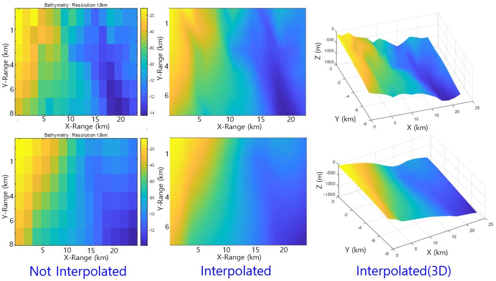
In order to check sensitivity to data sources between KTOPO and ETOPO1, we make the resolution of KTOPO be 1,800 m × 1,800 m (pick up every 60^th data) to get similar resolution to that of ETOPO1. Fig. 7 shows an example of selected bathymetry distributions of the two data sources, KTOPO (up) and ETOPO1 (down), in a region of depths 100 m ~ 1,300 m. From the left to the right, it gives 2D images of not interpolated and interpolated, and 3D image of interpolated, respectively. We can see that two data sets give similar patterns in general but different variations in detail.

Fig. 7.

(Color available online) Selected bathymetry distributions of different data sources in a region of depths 100 m ~ 1,300 m: (up) KTOPO, (down) ETOPO1.

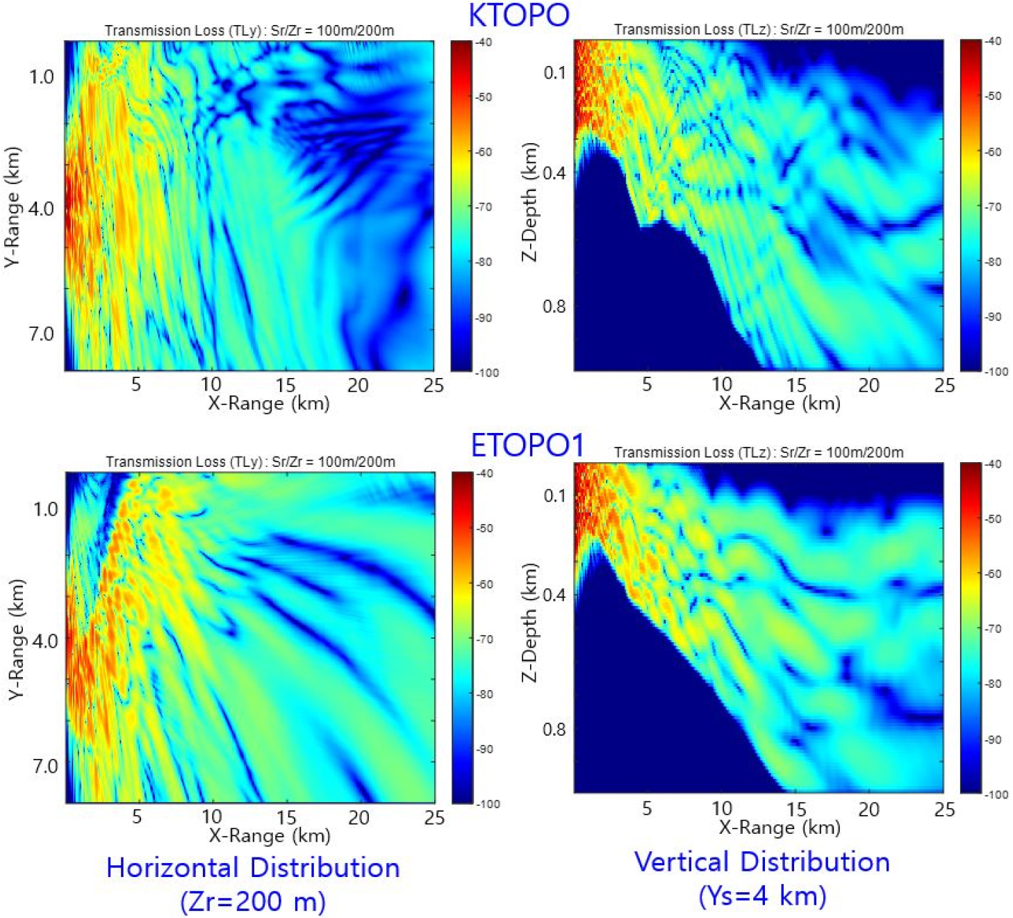
With these two data sets, we compare the results responding to different sources. Fig. 8 gives transmission loss distributions with different data sources in Fig. 7, KTOPO (up) and ETOPO1 (down). In the horizontal distributions (left) of receiver depth Zr = 100 m, we can see that general patterns are big different between the two figures.

Fig. 8.

(Color available online) Transmission loss distributions with different data sources in a region of depths 100 m ~ 1,300 m: (up) KTOPO, (down) ETOPO1.

Concerning the sensitivity to data resolutions, we do simulation with the KTOPO because we can change resolutions from high to low. Fig. 9 presents the bathymetry distributions of spatial horizontal grid 30 m (left), 300 m (center) and 1,800 m (right). The original images (top) show noticeable changes specially with 1,800 m grid, but the interpolated ones (bottom) do actually no changes. With the three data sets of resolution, we compare the transmission losses.

Fig. 9.

(Color available online) Selected bathymetry distributions of different data resolutions in a region of depths 100 m ~ 1,300m with the KTOPO: (up) not interpolated, (down) interpolated.

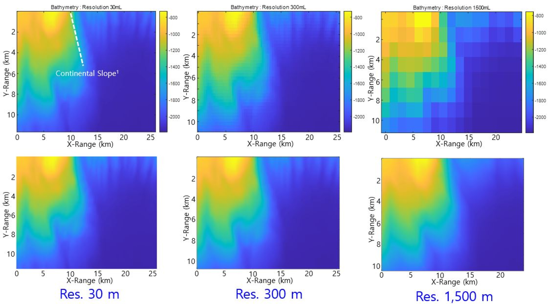
Fig. 10 shows transmission loss distributions with the bathymetry of different resolutions. All the figures show almost same patterns within propagating range (X) 0 km ~ 10 km, but that of resolution 1,800 m does different patterns after the range. This tendency is very similar to the patterns of bathymetry distributions themselves in Fig. 9. This is due to the fact that the model itself give (bilinear) interpolation over the input bathymetry data.^[2] The interpolation strategy is very reasonable because physical processes (current etc.) in water column give an effect to smooth out (interpolate) the big changes in bathymetry. Moreover, it is noticiable that the geoacoustic data used in the simulation are generally costly to acquire.

Fig. 10.

(Color available online) Transmission loss distributions with different data resolutions in a region of depths 100 m ~ 1,300 m with the KTOPO.

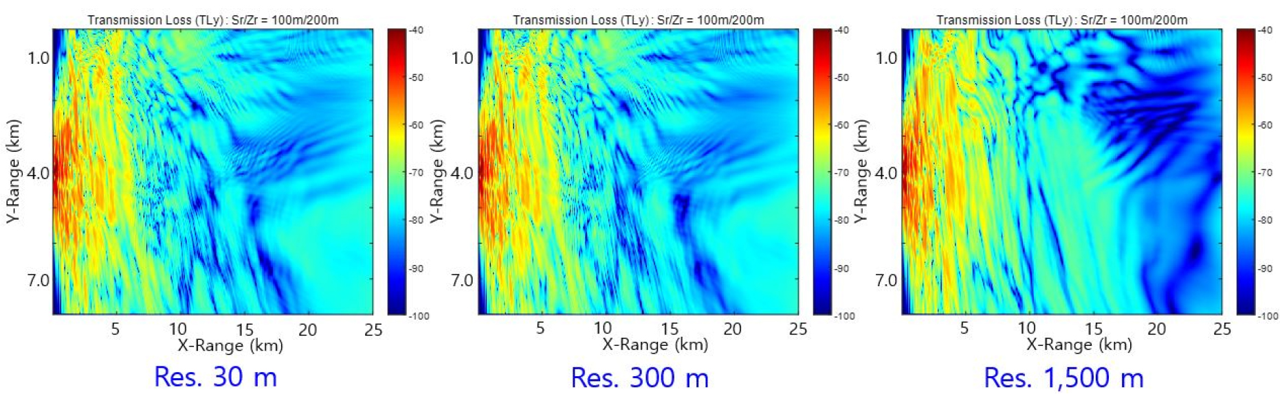
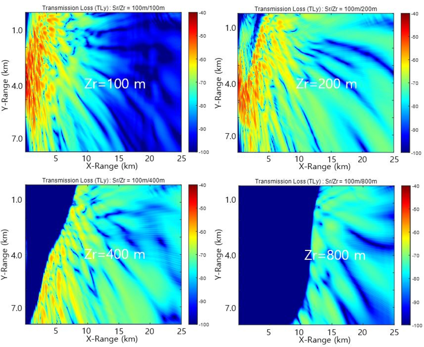
Fig. 11 shows transmission loss distributions with varying receiver depths as Zr = 100 m, 200 m, 400 m and 800 m in a region of depths 300 m ~ 2,200 m with the KTOPO. The regions of no data (Zr = 400 m and 800 m), where the water depths are less than receiver depths, consist of continental shelf and slope. We can see that transmission loss in the shallowest receiver depth (Zr = 100 m) increases dramatically after propagating range X = 15 km, indicating downward refractions of acoustic wave after continental slope.

Fig. 11.

(Color available online) Transmission loss distributions at four receiver depths (Zr = 100 m/200 m/400 m/800 m) in a region of depths 300 m ~ 2,200 m with the ETOPO1.

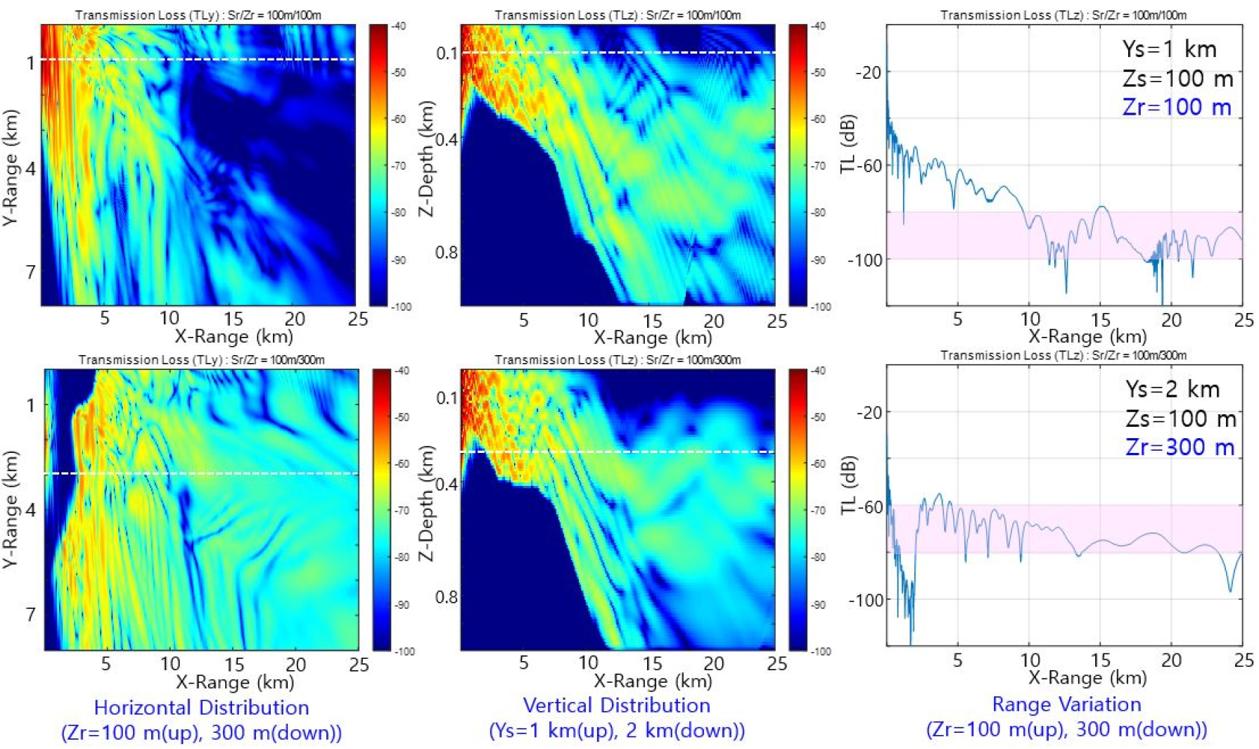
In Fig. 11, we can see that horizontal variations of transmission loss may be highly dependent on receiver depth. In oder to get an insight to operate variable depth sonars (for example line arrays) on a region of continental slope, we give a numerical example for different cross range positions of source with the same bathymetry data. Fig. 12 presents transmission losses when the source is located at the cross range Ys = 1 km (up) and 2 km (down). If we cut slices into the two cross ranges, we have vertical distributions as center figures in Fig. 12. The center figures show that we can hardly expect good detection performance after the continental slope within the receiver depths of surface to about 150 m because of big transmission loss. In the meanwhile, if the receiver is located at Zr = 300 m (down), it can keep good performance after the continental slope. If we cut slices into receiver depth Zr = 100 m and 300 m, we have transmission loss variation with propagating range X. We can see the two graphs show nearly 20 dB difference.

Fig. 12.

(Color available online) Transmission loss distributions on a continental slope in a region of depths 300 m ~ 2,200 m with the KTOPO. (up) source at Ys = 1 km, (down) source at Ys = 2 km.

In the situation where a source exists on the shallower region with continental slope, we can expect very long range propagation after a few bottom reflections on the continental shelf without surface reflections, i.e, Down- Slope Enhancement (DSE). Even if there exist DSE due to bathymetry conditions, there can also exist poor detection zone in the water column. Using this kind of information, sonar operators can decide their receiver depths for the best performance.

IV. Discussions

In solving cross-terms, Eq. (6) basically has the problem of numerical diverging due to the discontinuity of the numerical fields in the cross-term calculation. To avoid the problem, the model employs band-pass filter passing only the radiation spectrum part. When we let wavenumber be k, the filter can be expressed as –1/Alpha < k < 1/Alpha, where Alpha is positive real number.^[2] Smaller number of Alpha means more passing of energy. Through trial and error, we find normal calculation with Alpha value 1 ~ 4 in the sea around Korean peninsula. Fig. 13 illustrates an example of transmission losses with Alpha values of 8 (up) and 2 (down). For Alpha = 2 case, numerical calculation stops at the propagating range X = 13.3 (right), where continental slope ends (center). In the propagating range 13.2 km ~ 25 km, horizontal and vertical distributions are the images replaced with those of Alpha = 8 for comparison.

Fig. 13.

(Color available online) Transmission loss distributions with variable filtering coefficients (Alpha) where the source is located at Ys = 2 km, Zs = 100 m. (up) Alpha = 8, (down) Alpha = 2.

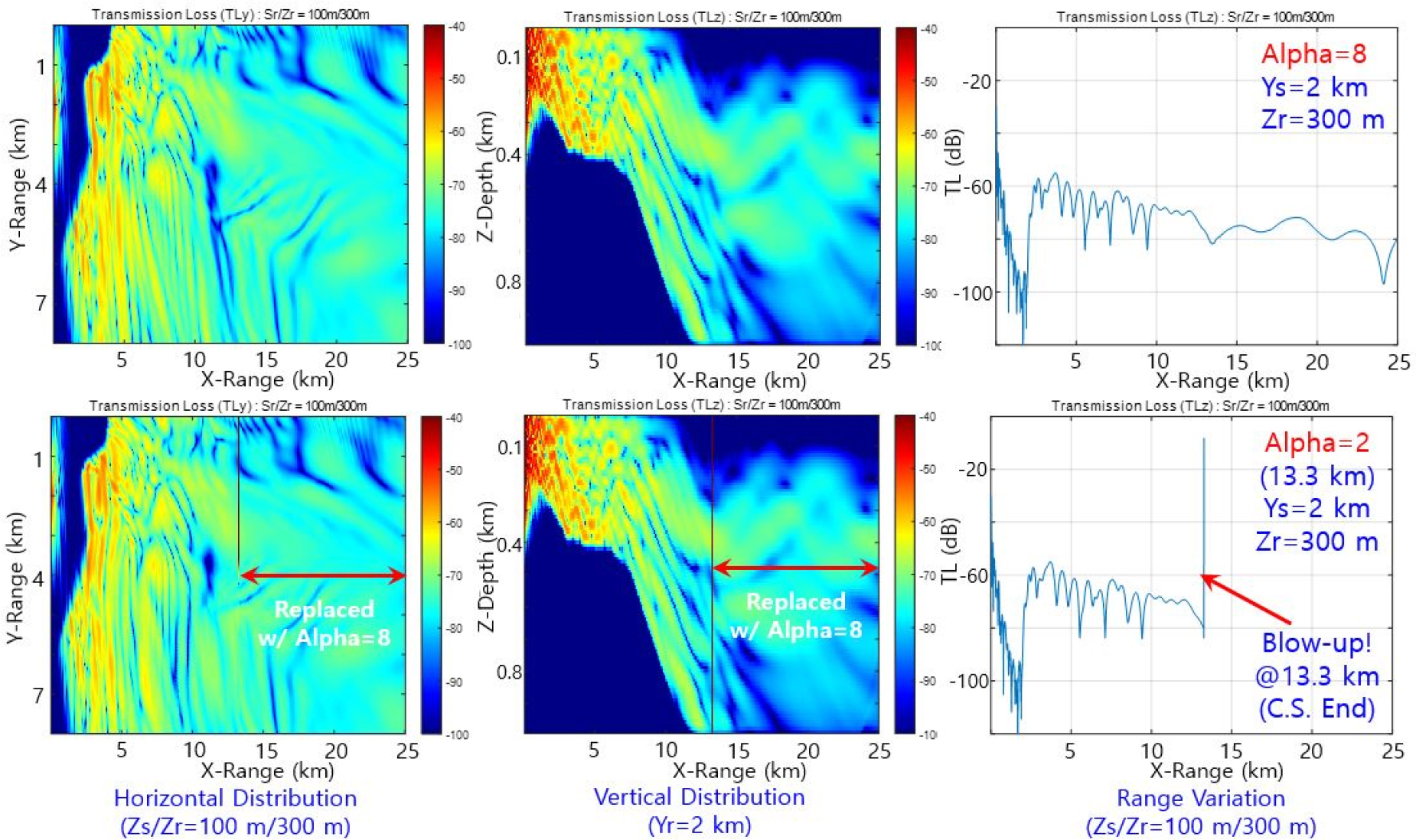
For avoiding numerical diverging from big spatial changes of bathymetry, the model may need some criteria on proper Alpha value in pre-processing the bathymetry data as input.

Another issue is the modeling of horizontal refractions due to 3D distributions of SSPs in water such as fronts and eddies. To simulate the 3D effect of SSPs, the model needs improvement to allow SSP in each 2D grid. This version (cuSPE0.9) adopts multiple SSPs only in the propagating range X, assuming same SSP in the crossing range Y at each point X.

V. Conclusions

This paper examines the applicability of the 3D model, cuSPE0.9, based on the parabolic equation in simulating horizontal refractions due to bathymetry distribution.

Assuming the CW source of 75 Hz at 100 m depth and artificial bathymetry shapes (‘V’, inverse ‘V’, and wedges), we can see the horizontal curved patterns of the transmission loss on the horizontal plane.depending on the bathymetry slope. The curved fronts are slanted toward to shallower depth region. The degree of curving increases with bathymetry slope increased. For fixed bathymetry slope, the slope of transmission loss patterns shows non- linear increase with the propagating range increased. Comparing the approximate results by cuSPE0.9 with those of full solution, we can see the two results show actually same patterns and absolute values.

Another simulations with real bathymetry data of different sources in regions of the depths of 100 m ~ 2,200 m, East Sea of Korea, we can notice that the model is somewhat sensitive to data sources but little sensitive to resolution of data source selected because it employs the bilinear interpolation scheme in pre-processing the bathymetry data.

In conclusions, the model is applicable to simulating horizontal refractions of acoustic waves responding to bathymetry variations. To be operational in such as ocean surveillance systems, the model needs some improvements to adopt 3D SSPs in water. To avoid numerical diverging at sharp bathymetry variation points, the model needs to suggest criteria on proper filtering coefficient estimated from such as horizontal gradient of depth or give a proper interpolation scheme to mitigate sharp bathymetry variations.