

I. Introduction
II. MoM Technique for a 2D cylinder in free-field
III. MoM Technique for a 2D cylinder partially buried on a flat interface
IV. Conclusions
I. Introduction
Although the investigation of the scattering of sound by partially buried object in sediment has been performed experimentally,[1] and theoretically,[2] the development of fast numerical methods could be helpful for giving insight into aspects of the scattering for a partially buried object. Method of Mements (MoM) is a kind of numerical technique assuming the object is composed of small segments which has a step-function like impulse response.[3] MoM is a fast and accurate numerical approach especially in the scattering problem for a complete smooth object. However, when the object is suddenly trucated by the interface, implementation of the MoM technique for the scattering problem is questioned. This work examines the application and the testing of the MoM to a simple case when the sound is incident and is backscattered from the 2D rigid cylinder truncated by a soft or rigid flat interface. In such case, backscattering amplitude from the cylinder is greatly affected by the reverberation from the interface.[4] In the current study, MoM technique is applied by combing the scattering from the object with the reverberation from the interface.
II. MoM Technique for a 2D cylinder in free-field
 and
and  , and
, and  is cylinder radius.
Generally, the acoustically scattered pressure by a two dimensional smooth cylinder is given as follow in the  convention:[5]
 (1)
(1)
where  is the scattered pressure,
  is the kernel, and
  is a zeroth-order Hankel function of the second kind. Vector
  represents the observed direction,
  means the integrated segments location, and
  is the area of the cylinder that the segments are integrated. The basic concepts of the MoM is approximating the kernel
  by using the propagator
  and the incident pressure
  . Once the kernel
  is obtained, the scattered pressure
  can be calculated from Eq.(1). At the surface of the cylinder, rigid acoustical boundary condition is imposed, which is
  . Because
  , on the surface of the rigid cylinder with the radius of
  , the following relationship is satisfied:
 (2)
(2)
Thus, substituting Eq.(1) into the r. h. s. of Eq.(2),
 (3)
(3)
where the subscript A represents the surface of the cylinder and 
 . For a convenience, the kernel


 was introduced here where
  is cylinder radius. Gradient of the Hankel function with respect to the coordinates
  is obtained as:
 (4)
(4)
When the observation point is arbitrary location on the surface of the cylinder as shown in the geometry of Fig. 1,  ,
,  ,
,  , and the normal vector on the surface,
  , are calculated as:
 (5a)
(5a)
 (5b)
(5b)
 (5c)
(5c)
 (5d)
(5d)
Then, normal derivative of Hankel function with respect to the coordinates  becomes:
 (6)
(6)
thus, Eq.(3) is expressed as:
 (7)
(7)
Introducing the kernel  as a superposition of the unit-step basis functions such as:
 (8a)
(8a)
 (8b)
(8b)
then, for a given incident pressure at m-th cell, Eq.(7) is discretized as:

Eq.(9) tells that a given incident pressure at m-th cell can be expressed as the product of unknown coefficient  and the integration of
  within n-th cell, which is displayed as an element of the impedance matrix in Eq.(11). Therefore, for the N-numbers of cases from m = 1 to m = N, Eq.(9) constitutes following matrx equa-tion
|
Fig. 2. Geometry of the MoM elements on the cylinder. Indices for the observed cell and the local cell are denoted as |
 and
and  respectively.
 (10)
(10)
where  is
is  incident matrix,
  is
is  impedance matrix, and
  is
is  unknown coefficients describing the kernel
  . When the kernel
  is discretized on the surface of the cylinder, in order to give accurate results on the scattering form function,
  should satisfy the condition of
  where
where  is wavenumber- radius product in propagating medium. Such condition can be derived by the Nyquist sampling theorem.
Fig. 2 shows the geometry to calculate the matrix elements of  and
and  . Locations of the centers of the m-th cell and the n-th cell are denoted as
  and
and  respectively. Distance between centers of m-th cell and n-th cell is denoted as
  . At the location of m-th cell, normal derivative of the incident pressure can be approximated as the value at the center of m-th cell if size of the cell is sufficiently small compared to the wavelength of the incident pressure. Thus, for the m-th cell, normal derivative of the incident pressure becomes:
 (11)
(11)
where incident direction is along - as shown in Fig. 2. Calculation of the elements of the impedance matrix
  are different for the off-diagonal elements where
  and diagonal elements where m = n. The result of the calculation of impedance matrix which is independent of the incident direction is as follows:[3]
 (12)
(12)
Once matrix  is obtained by
  , the scattered pressure can be evaluated by substituting the kernel
  with the matrix
  in Eq.(1). For the far-field scattering, far-field pressure can be approximated by using following approximation for the Hankel function at large argument:[6]
 (13)
(13)
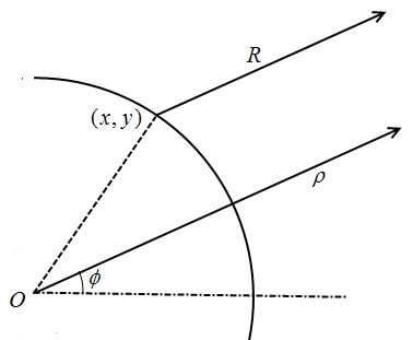
Because distance R from the point scattered to the observed point can be approximated as 

 at the far-field as shown in Fig. 3 where angle
  is direction of the observed point, the resulting scattered pressure can be expressed as

Hence, using the above expression, calculating the scattering amplitude f,
 (15)
(15)
and normalizing  with respect to
  , the dimensionless form function
  is obtained as
 (16)
(16)
where  is wavenumber radius product. In Eq.(16), the direction of the far-field is determined by the angle
  and the incident pressure determines the value of
  from Eq.(10). In case of the backscattering, the incident angle is identical to the angle
  .
.
The exact solution of the scattering amplitude of a 2D cylinder for the broad side incidence is well known as follows in  convention:[7]
 (17)
(17)
Fig. 4 shows the comparison of the MoM results in Eq.(16) with the exact solution in Eq.(17) for four different values of  as a function of the scattering direction,
  . Black dots represent the result of MoM simulation and the solid lines are the exact solution.
  values range from 5 to 20. All MoM simulations were done using 1000 number of equal line segments along the circumference of the cylinder, which satisfies the condition of
  . In evaluating Eq.(17), the infinite series of Bessel function or Hankel function were substituted as the finite series with the proper choice of the truncation which is the maximum value of index m. The truncation limit
  was chosen as
  which is the sufficient value that does not affect the shape of the graph.[8] Around the scattering angle of
  , maximum peaks are observed, which is the effect of the forward scattering by the incident pressure. MoM results are consistent with the exact solution, however, at higher value of
  , the result is not accurate. Some abnormal behavior of the MoM simulation happens at special values of
  . Such deviation between MoM results and exact solution comes from the numerical accuracy of the Bessel function implemented in MATLAB. Evaluation of Bessel function is critical to obtain impedance matrix as shown in Eq.(12). Over most values of ka, expression in Eq.(12) is enough to give accurate results on the scattering amplitude. However, for a certain value of ka, evaluation of Bessel function in MATLAB is not as accurate as other programs. When the same MoM calculation is performed for ka=20 with older version ofMATLAB, errors between MoM results and the exact solution become much larger than Fig. 4(d) although such comparison was not shown in the current study. It is not also shown here that when more accurate expression of impedance matrix was adopted, the errors between MoM results and the exact solution was suppressed.
 such as (a)
  , (b)
, (b)  , (c)
, (c)  , and (d)
  . MoM shows the overall good agreements with the exact solution. But, at the special value of
  , it deviates severely from the expectation.
III. MoM Technique for a 2D cylinder partially buried on a flat interface
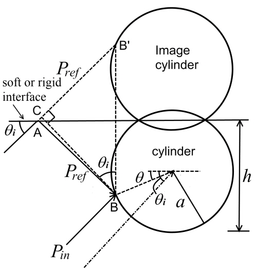
When considering the scattering for a buried object on a flat interface, two incident pressure are considered as shown in Fig. 5 which shows the partially buried cylinder and its image cylinder. Grazing angle is denoted as  . At a given point B on the surface of the cylinder, two pressures contributes its total incident pressure. One is the directly incident pressure from the plane wave source and the other is the reflected pressure from the flat interface. In the current study, two kinds of flat interfaces are considered: soft interface where total pressure vanishes and the rigid interface where the normal derivatives of the total pressure vanishes, which modifies the phase of the reflected pressure from the flat interface.
From Fig. 5, incident pressure  onto the point B, in
  convention, is expressed as
 . Path difference between
  and
and  is the same as the length
  . Length
  is the same as
  . So, the reflected pressure
  , where

 and the positive and negative signs in front of
  come from the rigid and soft boundary conditions of the interface respectively. Therefore the total pressure onto the point B becomes
 . At a given point B on the surface of the cylinder, two pressure contributes its incident pressure. One is directly incident pressure from the source and the other is reflected pressure by the flat interface. Hence, total incident pressure is the sum of the directly incident pressure and the reflected pressure with the phase consideration. For the backscattering, the scattered pressure is the exact opposite process of the incident case.
 less than
  .
.where  and (+) for rigid interface and (-) for soft interface. Then the incident matrix
  is the normal derivative of the total incident pressure in Eq.(18). But, we need to specify which line segments of the cylinder is buried and is not exposed. Thus, the line segments of the buried elements of the
  are considered as zeros as follows.

When Eq.(19) is substituted into Eq.(10), matrix  is obtained for the case of the scattering by a partially buried cylinder on a flat interface. Once unknown coefficient,
  , is obtained, backscattering form function is obtained just making the scattering process exactly opposite to the inci-dent process. Thus, total backscattered pressure consists of the pressure backcattered from the surface of the original cylinder and the scattered pressure toward the interface which is followed by the reflection from the interface to the plane wave source. Therefore, from the same approxima-tion and the processes in Eqs.(14)~(16), the dimensionless form function
  for a partially buried cylinder on a flat interface is

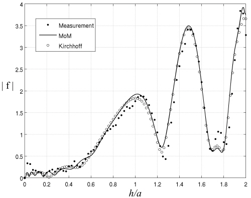
Fig. 6 shows the comparison of the experimental measurements of the backscattering form function for a partially exposed cylinder on an air-water interface with the analytic solution by Kirchhoff approximation[2] and the MoM simulation with 360 elements using Eqs.(19) and (20). For the detail experimental setup and the measurements, see Reference 2. Horizontal axis is the order of the exposure of the cylinder through the interface, which is normalized by  (see Fig. 5). The data were taken at 160 kHz with 30 degree grazing incidence (
 °) which are indicated as black dots. Because measurements were carried out for an air-water interface, soft boundary condition was used in the MoM simulation, thus, negative sign was adopted in Eqs.(19) and (20). MoM simulation is solid line and the analytic solution is denoted as blank circles. Both methods matches well with the measurem ents and show the same behavior with each other, however, at small h, MoM simulation is more oscillatory than the analytic solution.
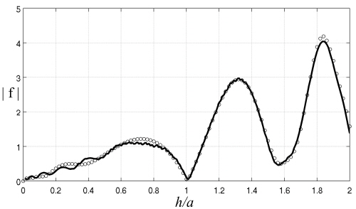
Fig. 7 shows the Kirchhoff approximation and MoM simulation for the backscattering amplitude with rigid interface as a function of the h at 140 kHz. Solid lines represent the MoM simulation, and blank circles are the Kirchhoff approximation. Through all h of the cylinder, two methods show good agreements with each other. As shown in Fig. 6, MoM results are more oscillatory than the Kirchhoff approximation for small h.
|
Fig. 7. Comparison of backscattering amplitude by the MoM simulation (solid) and the Kirchhoff approximation (blank circle) when the flat interface is rigid at the driving frequency of 140 kHz. |
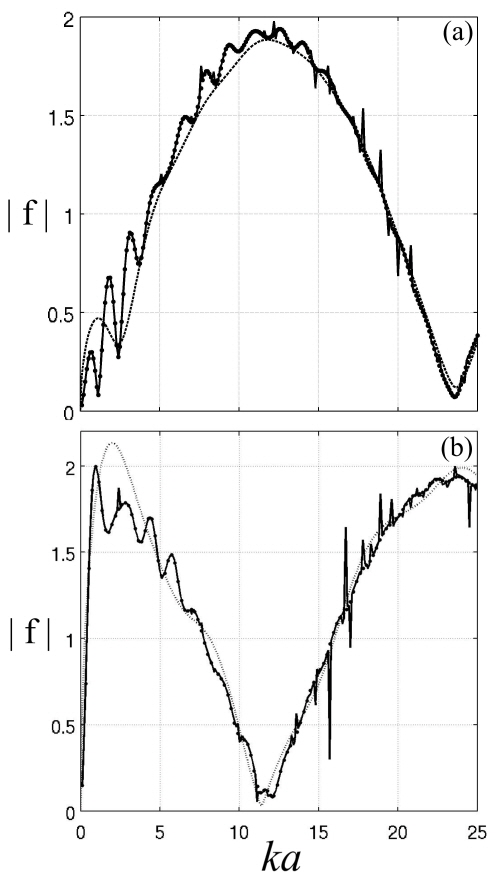
 through (a) soft flat interface and (b) rigid flat interface. The horizontal axis is
  and vertical axis is the normalized backscattering amplitude. Incident angle of each picture is 30 degree. MoM results are much closer to the exact solution than the Kirchhoff approximation, however, at some value of the
  it returns the strange spikes.
As shown in Figs. 6 and 7, MoM simulation was performed for the partially submerged cylinder on a flat interface. Through the comparison of the MoM with the Kirchhoff approximation and measurements, we saw it was useful to describe a partially submerged cylinder. An exact solution can be calculated for the special case when the cylinder is halfway exposed, that is  . This problem was solved by Twersky[9] and derivation of the exact solution was shown in Reference 2. Figs. 8(a) and 8(b) show comparisons of the exact scattering amplitude with the Kirchhoff approximation and the MoM simulation with 360 elements as a function of
  from 0 to 25 at given incident angles of 30 degree when the cylinder is halfway exposed on a flat soft interface and on a flat rigid interface respectively. The measurements are denoted as black dots, the dashed line is Kirchhoff approximation, and the solid line represents MoM simulation. The exact solution shows more oscillatory behavior than the Kirchhoff approximation and is very close to the MoM simulation. MoM results correspond to the exact solution regardless of low or high value of
  . But the strange spikes for certain
  values are seen. This is the same phenomena when the exact solution of the single cylinder scattering was compared with the MoM as shown in the Fig. 4. Sometimes the MoM returns severely deviated result which might be caused by the numerical convergence of the method. If such anomaly is fixed, MoM is more accurate method than Kirchhoff approximation regardless of rigid or soft boundaries of interface.
IV. Conclusions
The MoM simulation for the backscattering by a partially buried rigid cylinder on a soft or rigid flat boundary was presented. Comparing to the analytic solution calculated by the Kirchhoff approximation,[2] MoM technique for the problem shows the good agreements with the measurements and the exact solution as well as the Kirchhoff approximation. A key issue in the scattering by a partially buried object on a seabed is that the reverberation from the seabed greatly affects the scattering amplitude, which was shown analyti-cally[2] in the previous study and numerically in the current study. Thus, the MoM technique presented in the currrent study can be applied to any shape of the smooth objects that are partially buried on a seabed if the reverberation from the seabed is known or well characterized.
