Vector quantization as a post-training regularizer for passive underwater acoustic target classification

Jaeyeong Hwang; Sangmin Lee; Yoonchang Han; Donmoon Lee; Do Kyung Shin; Seung Hwan Kim; Min Young Kim; Young Dae Kim

doi:10.7776/ASK.2026.45.4.333

Preview

The Journal of the Acoustical Society of Korea. 31 July 2026. 333-342
https://doi.org/10.7776/ASK.2026.45.4.333

Vector quantization as a post-training regularizer for passive underwater acoustic target classification

수동 수중 음향 표적 분류를 위한 사후 학습 정규화기의 벡터 양자화

Jaeyeong Hwang¹

Sangmin Lee¹

Yoonchang Han¹

Donmoon Lee¹^*

Do Kyung Shin²

Seung Hwan Kim²

Min Young Kim²

Young Dae Kim²

황 재영¹

이 상민¹

한 윤창¹

이 돈문¹^*

신 도경²

김 승환²

김 민영²

김 영대²

¹Cochl, Inc.

²LIG Defense & Aerospace

^{*Corresponding Author}

License (open-access, http://creativecommons.org/licenses/by-nc/4.0/):

This is an Open Access article distributed under the terms of the Creative Commons Attribution Non-Commercial License which permits unrestricted non-commercial use, distribution, and reproduction in any medium, provided the original work is properly cited.

ABSTRACT

This study proposes a Vector Quantization (VQ) based regularizer to mitigate the overfitting of overparameterized deep learning models in underwater acoustic target recognition, where training data are scarce. We introduce a discrete bottleneck layer that is applied after a classification network has been fully trained on the target task. The bottleneck compresses the continuous representation into a finite codebook and reconstructs it before classification. To ensure stable optimization, we incorporate an autoencoder initialization and a model selection rule based on validation loss and codebook usage. Using the ShipsEar dataset, the proposed method achieves 79.7 % accuracy on Residual Networks (ResNet)-50, outperforming the baseline by 4.8 % with lower training variance. Through ablation studies, we demonstrate that the discretization process, post-training setup, autoencoder initialization, and the proposed model selection rule are jointly necessary to achieve the regularization gains, showing its effectiveness as a representation level constraint for underwater acoustic classification under data scarcity.

Keywords

Passive sonar

Neural networks

Regularization

Vector Quantization (VQ)

Information Bottleneck (IB)

Vessel classification

본 연구에서는 데이터가 부족한 수중 음향 표적 인식 환경에서 신경망의 과적합을 완화하기 위해 벡터 양자화 기반의 정규화를 제안하였다. 이는 분류 네트워크가 목표 작업에 대해 학습된 후에 적용되는 이산 병목 층을 도입하는 것으로, 연속적인 임베딩을 유한한 코드북으로 압축한 후, 분류 단계 이전에 이를 재구성하는 방식으로 구현되었다. 추가로, 안정적인 최적화를 보장하기 위해 오토인코더 초기화와 코드북 사용량에 기반한 모델 선택 규칙을 제안하였다. ShipsEar 데이터셋에서 진행된 실험 결과, 제안 방식은 기존 Residual Networks(ResNet)-50 분류기 대비 4.8 % 향상된 79.7 %의 정확도를 달성하며 정규화 이득 측면의 효과성을 입증하였다. 또한, 이산 병목, 사후 학습, 오토인코더 초기화, 그리고 제안된 모델 선택 규칙은 효과적인 정규화를 달성하기 위해 모두 필요함을 입증하였다.

키워드

수동 소나

신경망

정규화

벡터 양자화(Vector Quantization, VQ)

정보 병목(Information Bottleneck, IB)

선박 분류

MAIN

I. Introduction
II. Proposed methods
2.1 Overview
2.2 Training and model selection
III. Experimental setup
3.1 Data preparation
3.2 Model architectures
3.3 Implementation details
IV. Results and discussions
4.1 Backbone capacity and generalization effectiveness
4.2 Parameter sensitivity
4.3 Ablation study
V. Conclusions

I. Introduction

Unlike in terrestrial environments, visual perception is severely limited underwater, making acoustic sensing such as sonar the primary medium for perception.^[1] Consequently, underwater acoustic target recognition is a key task in fields such as national defense, underwater surveillance, and marine monitoring.^[2] Traditionally, this task has been performed by trained human operators.^[3] However, this manual approach requires expensive training and suffers from performance degradation due to operator fatigue.^[4] These limitations have motivated the adoption of deep learning-based approaches as a more scalable alternative.^[5]

Deep learning models require massive training data, but acquiring such large datasets for the underwater domain is challenging. These challenges arise from high collection costs, military security regulations, and marine environmental regulations. Due to these constraints, publicly available underwater acoustic datasets are limited in both quantity and quality. For instance, ShipsEar, a dataset widely used in the academic community, consists of 90 audio recordings across 11 vessel types, amounting to only about 3 h of data in total.^[6] Even DeepShip, a relatively recently released large scale dataset, contains only about 47 h of data across 4 vessel classes.^[7] Compared to modern large scale deep learning models, which typically require tens of thousands of hours of speech or millions of images, these underwater datasets are relatively scarce. Consequently, modern large scale architectures that have driven recent breakthroughs in other domains cannot be effectively trained on such limited underwater data, and many works still rely on supervised training of smaller classification networks from scratch, resulting in representations that overfit to characteristics specific to the dataset.

Such data scarcity typically leads to overfitting. To mitigate this issue, various regularization strategies have been proposed, which can be broadly classified into three categories: optimization level regularizers, architecture level constraints, and representation level constraints. First, optimization level regularizers, such as weight decay,^[8] dropout,^[9] and label smoothing,^[10] impose constraints on the network’s parameters or soften target distributions. However, these are essentially indirect approaches, as they restrict the parameter space or smooth the loss landscape without directly limiting the information capacity of the learned features, and therefore struggle to effectively regularize overparameterized models.^[11] Second, architecture level constraints,^[12,13] such as employing smaller networks or low dimensional bottleneck layers, directly reduce model complexity. However, these approaches often constrain the expressive power of the model and limit the ability to leverage the rich, broadly applicable representations available from pretrained large models.

In contrast to these approaches, representation level constraints, often motivated by the Information Bottleneck (IB) principle, offer a more fundamental alternative.^[14] By explicitly restricting the flow of information through the network, these methods guide the model to retain only essential features relevant to the task. This bottleneck is typically implemented in two forms. Continuous approaches inject stochastic noise into the representation (e.g., the Variational Information Bottleneck^[15]), whereas Vector Quantization (VQ) introduces a discrete bottleneck by restricting representations to a finite codebook.^[16] VQ, in particular, has been widely studied in generative modeling and self-supervised pre-training. However, its potential as a direct regularizer for supervised classification, especially under data scarcity, remains underexplored.

In this paper, we propose VQ as a post-training regularizer for training classifiers on low-resource underwater acoustic datasets. By inserting a discrete bottleneck into a pretrained classifier and continuing optimization on the same task, our method compresses the learned representation, discarding task-irrelevant information and thereby improving generalization. The main contributions of this paper are summarized as follows:

First, we propose a training method that uses VQ as a regularizer. To overcome the optimization instability of discrete bottleneck training, we introduce an Autoencoder (AE) initialization strategy and a model selection rule based on codebook usage. Experimental results confirm that discretization, the post-training setup, AE initialization, and the proposed model selection rule are jointly necessary to achieve the observed generalization gains.

Second, we statistically validate the efficacy of the proposed method through extensive experiments on the ShipsEar dataset. Our analysis further reveals that the regularizing effect of the discrete bottleneck is most pronounced when the model is large relative to the available training data, which is the typical setting for underwater acoustic recognition.

II. Proposed methods

2.1 Overview

We propose a VQ based regularizer that inserts a discrete bottleneck layer to compress the high level embedding vector $h$ (Fig. 1). Unlike conventional regularization schemes, our method is applied after the network has been fully trained on the target task. The discrete bottleneck acts as a regularizer by constraining the information flow through a finite codebook and enforcing discrete embeddings. In this context, “post-training regularizer” denotes a procedure that structurally compresses representations for the original task, which differs from conventional fine-tuning in that it conducts further training under the same objective.

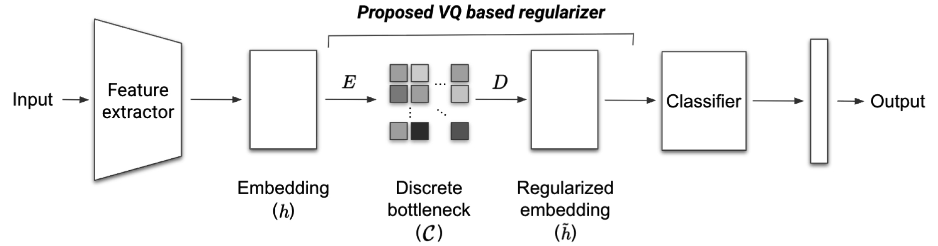
https://cdn.apub.kr/journalsite/sites/ask/2026-045-04/N0660450401/images/ASK_45_04_01_F1.jpg

Fig. 1.

(Color available online) An overview of our proposed VQ based regularizer. A feature extractor produces a high level embedding $h$ , which is mapped by an encoder $E$ to its nearest entry in a discrete bottleneck $C$ ; a decoder $D$ then reconstructs a regularized embedding $\tilde{h}$ that is fed into the classifier. The proposed VQ based regularizer consists of an encoder $E$ , a Discrete bottleneck $C$ , and a decoder $D$ , which is inserted between the feature extractor and the classifier of a pretrained network.

Our overall pipeline consists of four steps: (i) training the classification network on the target task, (ii) inserting the VQ bottleneck layer, initializing its encoder and decoder weights using an autoencoder and initializing the codebook with embeddings randomly sampled from the training set, (iii) continuing to train the VQ augmented network on the target task, and (iv) selecting the optimal model based on codebook usage and validation performance.

2.2 Training and model selection

We follow the standard Vector Quantized Variational Autoencoder (VQ-VAE) formulation,^[16] which includes Straight-through gradient estimation and Exponential Moving Average (EMA) codebook updates. The bottleneck consists of an encoder $E$ , a codebook $C = \{e_{1}, \dots, e_{K}\} \subset ℝ^{d}$ , and a decoder $D$ . The encoder projects a high level embedding $h$ into $z_{e} = E (h)$ , which is then quantized to its nearest codebook entry $z_{q} = \underset{e_{i} \in C}{\arg \min} {||z_{e} - e_{i}||}_{2}$ and decoded into a regularized high level embedding $\tilde{h} = D (z_{q})$ . The encoder, the decoder, and the codebook follow distinct update rules. The decoder $D$ is trained with the classification loss via gradient descent. The encoder $E$ and the codebook $C$ are aligned through a pair of complementary mechanisms: the encoder is pulled toward the codebook by the commitment loss, while each codebook entry is pulled toward the encoder by an EMA over its assigned encoder outputs. The encoder additionally receives classification gradients through the Straight Through Estimator (STE), which bypasses the non-differentiable quantization step. The commitment loss and the EMA update are defined as follows:

(1)

L_{commit} = {||z_{e} - sg (z_{q})||}_{2}^{2},

(2)

N_{k} \leftarrow γ N_{k} + (1 - γ) n_{k},

(3)

M_{k} \leftarrow γ M_{k} + (1 - γ) m_{k},

(4)

c_{k} \leftarrow M_{k} / N_{k},

where $n_{k}$ and $m_{k}$ are the number of mini-batch encoder outputs assigned to code $c_{k}$ and their sum, $N_{k} \in ℝ$ and $M_{k} \in ℝ^{d}$ are the exponential moving averages of $n_{k}$ and $m_{k}$ , respectively. $γ \in (0, 1)$ is the EMA decay rate, $sg (\cdot)$ is the stop-gradient operator.

Finally, the training objective for the proposed method is

(5)

L = L_{cls} + λ_{commit} \cdot L_{commit},

where $L_{cls}$ is the classification (cross entropy) loss for the target task and $λ_{commit} \geq 0$ is the weight for the commitment loss.

We select the optimal model based on validation loss and codebook usage. Since the codebook is randomly initialized from the training set, all entries are initially active. As training progresses, only a subset of entries continues to be assigned encoder outputs, while the rest become inactive, which means no training sample is mapped to them. This indicates that the codebook has converged to a compact set of prototypes. Accordingly, we monitor the codebook usage, and once it drops below 100 % with some entries becoming inactive, we select the model with the best validation loss. The effectiveness of this proposed approach is analyzed in Section 4.3.

III. Experimental setup

3.1 Data preparation

We used the ShipsEar dataset,^[6] a public dataset for sonar classification. ShipsEar is a dataset of underwater ship sounds collected directly from hydrophones. It consists of 90 recordings for 11 types of ships, and the total length of the sound sources is approximately 3 h. The recording durations range from 9.9 s to 682.6 s.

Following the previous studies,^[17,18] we select 9 vessel classes in the ShipsEar dataset,^[6] yielding a total of 83 recordings. The recordings are then split into training and test sets at the recording level (62 recordings for training and 21 for testing). Each recording is segmented into 30 s windows with 15 s overlap, resulting in 587 segments in total. For every experimental run, 15 % of the training recordings were randomly held out as a validation set.

Consequently, 53, 9, and 21 recordings are allocated to the training, validation, and test sets, respectively. Although the combined number of training and validation segments is fixed at 471, the number of validation segments varies from 57 to 157 depending on the random sampling. The test set contains 116 segments.

Following the previous study,^[17] we compute 300-bin log-Mel spectrograms^[19] with Fast Fourier Transform (FFT) size 2,048 and hop size 1,024, covering frequencies up to 16 kHz. All recordings are resampled to 32 kHz prior to feature extraction. We do not apply any data augmentation.

3.2 Model architectures

We refer to the classifier trained without the VQ based regularizer as the base classifier, which serves both as the starting point for our post-training procedure and as the baseline for comparison. The base classifier adopts a generic Convolutional Neural Networks (CNN)-based audio classification architecture, in which a CNN backbone takes the log-Mel spectrogram as input and a final global average pooling layer extracts a vector embedding. A fully connected layer with Rectified Linear Unit (ReLU) activation projects the pooled vector into a 256-dimensional high level embedding $h$ . A 9-class classification head with softmax activation produces the prediction. We use ResNet-50^[13] as the feature extraction backbone, where overfitting is most severe and the regularization effect is most pronounced. Smaller backbones (ResNet-18,^[13] MobileNetV2^[12]) are analyzed in Section 4.1.

The VQ bottleneck is inserted between the high level embedding $h$ and the classification head. The encoder and the decoder are fully connected layers with linear activation. We set the bottleneck dimension to $d$ =32 and the codebook size to $K$ =64. The decoder reconstructs the quantized representation back to a 256-dimensional regularized high level embedding $\tilde{h}$ , so that the classification head and its input dimension remain identical to those of the base classifier, isolating the effect of the VQ based regularization.

3.3 Implementation details

All training uses the Adam optimizer^[20] with learning rate 10^–4 and batch size 64. The base classifier is trained for 50 epochs with categorical cross entropy loss, and the model with the lowest validation loss is selected. For the proposed VQ layer, the bottleneck encoder and decoder are first initialized with Mean Squared Error (MSE) loss using an autoencoder for 50 epochs while freezing the rest of the network, then the entire network is trained for an additional 100 epochs with $λ_{c o m m i t}$ =0.25 and EMA decay 𝛾=0.99. The optimal model is then selected based on the codebook usage and validation loss, as described in Section 2.2.

All experiments are repeated 10 times with different random seeds and validation splits, and we report the mean and standard deviation of test accuracy across runs. All backbone networks (ResNet-50, MobileNetV2, ResNet-18) are initialized with ImageNet-pretrained weights following the previous study.^[17]

IV. Results and discussions

4.1 Backbone capacity and generalization effectiveness

We evaluate the baseline performance across three models: ResNet-50, MobileNetV2, and ResNet-18, which have 25M, 3.4M, and 11M parameters, respectively. The baseline accuracies are 0.749, 0.759, and 0.788, respectively. Our implementation results are similar to those of the previous study,^[17] with a minor difference of less than 0.02. To statistically validate the performance differences, we conduct two-tailed paired t-tests across 10 independent runs for each condition.

Comparing the baseline and the proposed method, the results change depending on the model size (Fig. 2). The largest model, ResNet-50, shows the largest improvement, achieving a gain of 4.8 %. As a result, the accuracy after applying the VQ based regularizer increases with model size. Furthermore, the regularizer reduces the standard deviation of ResNet-50 from 0.0457 to 0.0169, making the training much more stable.

https://cdn.apub.kr/journalsite/sites/ask/2026-045-04/N0660450401/images/ASK_45_04_01_F2.jpg

Fig. 2.

(Color available online) Performance comparison across backbones. Statistical significance is assessed by paired t-test against the baseline, where ** indicates p < 0.01.

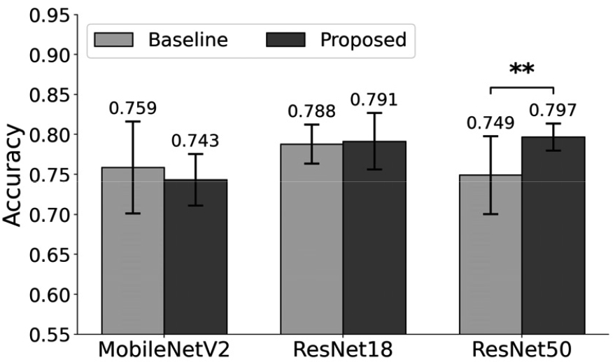
We hypothesize that this capacity dependence occurs because a bottleneck works by compressing existing information. Therefore, a larger backbone model is more advantageous because it can extract more abundant features before the bottleneck. Combining a large model with our VQ based bottleneck allows the regularizer to filter out features irrelevant to the task, while preserving only the information essential to the task.

4.2 Parameter sensitivity

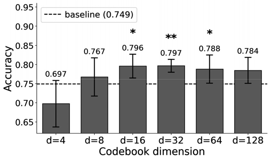
The performance of the VQ based regularizer depends on the bottleneck dimension, showing stable improvements within specific ranges of the hyperparameters. As shown in Fig. 3, when the codebook dimension $d$ is in the range of 16 to 128 with the codebook size $K$ =64, the proposed method consistently outperforms the baseline, with $d$ =16 and $d$ =32 achieving the most significant gains. This implies that an excessively small dimension ( $d$ =4) restricts the representation capacity, whereas larger dimensions do not significantly degrade the regularization effect.

https://cdn.apub.kr/journalsite/sites/ask/2026-045-04/N0660450401/images/ASK_45_04_01_F3.jpg

Fig. 3.

(Color available online) The accuracy across the codebook dimensions $d$ with the codebook size $K$ =64. Statistical significance is assessed by paired t-test against the baseline, where * and ** indicate p < 0.05 and p < 0.01, respectively.

In contrast to the sensitivity to the codebook dimension $d$ , Fig. 4 reveals that changing the codebook size $K$ across 32, 64, and 128 results in similar accuracy profiles, indicating that the model is highly insensitive to $K$ as long as $d$ is appropriately configured. This occurs because the proposed method selectively utilizes a subset of codebook entries, ensuring that performance is not constrained by the redundant capacity of a larger $K$ .

https://cdn.apub.kr/journalsite/sites/ask/2026-045-04/N0660450401/images/ASK_45_04_01_F4.jpg

Fig. 4.

(Color available online) The accuracy across the codebook size $K$ with the codebook dimension $d$ =32. Statistical significance is assessed by paired t-test against the baseline, where * and ** indicate p < 0.05 and p < 0.01, respectively.

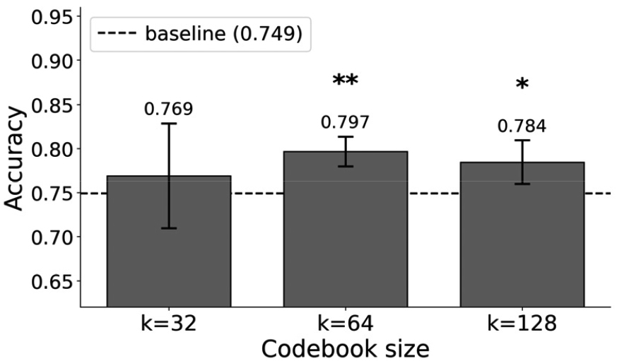
These results indicate that the codebook dimension and size are most effective within specific ranges. When the parameters become too large ( $d$ ≥64), the regularization effect weakens, causing performance to revert toward the baseline. On the other hand, when the bottleneck scale is too small ( $d$ ≤8), a noticeable performance drop occurs, as a smaller dimension results in information loss.

From a network design perspective, these findings suggest that the codebook dimension $d$ serves as the primary hyperparameter controlling the bottleneck, while the codebook size $K$ has minimal impact on performance, so optimization can focus on tuning the dimension $d$ .

4.3 Ablation study

Table 1 presents an ablation study to verify the effectiveness of each proposed component. Here, row (a) denotes the baseline model, while row (f) represents our proposed method with all modules integrated. The results demonstrate that the effectiveness of our approach derives from the synergistic combination of these design choices.

Table 1.

Ablation of the four proposed components on ResNet-50 with $d$ =32, $K$ =64. The top row represents the ResNet-50 baseline without the VQ based bottleneck. Here, AE, PT, DB, and MS denote Autoencoder initialization, Post-training regularization, Discrete bottleneck, and the Model selection rule, respectively. Statistical significance is assessed by paired t-test against the baseline, where ** indicates p < 0.01.

Row	AE	PT	DB	MS	Accuracy
(a)	×	×	×	×	0.7491 ± 0.0457
(b)	×	✔	×	×	0.7509 ± 0.0782
(c)	×	×	✔	✔	0.7397 ± 0.0709
(d)	×	✔	✔	✔	0.4759 ± 0.1309**
(e)	✔	✔	✔	×	0.7621 ± 0.0596
(f)	✔	✔	✔	✔	0.7966 ± 0.0169**

1. The effect of the proposed model selection rule: As shown in rows (e) and (f) of Table 1, conventional model selection using validation loss reduces the accuracy from 0.7966 to 0.7621. This shows that our strategy is helpful for isolating the regularized state from the unstable early phase of training. As illustrated in Fig. 5, during the early stages of post-training, the highest validation accuracy does not align with the optimal test accuracy. However, as training progresses and codebook selection occurs, the validation metric becomes a reliable guide for model selection.

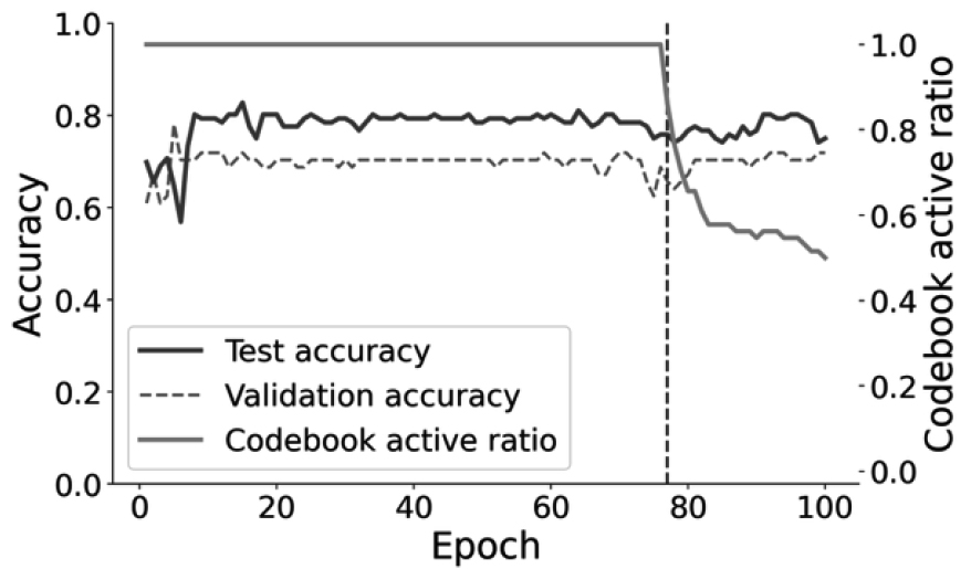
https://cdn.apub.kr/journalsite/sites/ask/2026-045-04/N0660450401/images/ASK_45_04_01_F5.jpg

Fig. 5.

(Color available online) The validation accuracy, test accuracy and codebook active ratio during training in row (f) of Table 1.

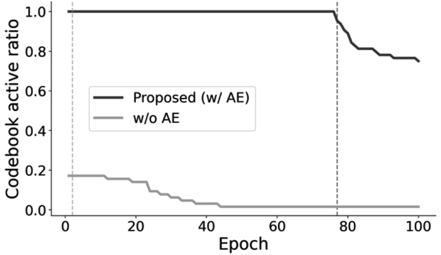
2. The effect of the codebook initialization using an autoencoder: As shown in row (d) of Table 1, omitting autoencoder initialization drops the accuracy to 0.4759 even when both post-training and the discrete bottleneck are active — a performance degradation relative to the baseline. This drop occurs because, as shown in Fig. 6, unlike the autoencoder initialized model which effectively utilizes the necessary entries from the full codebook, the model without autoencoder relies on only a tiny fraction of the codes right from the beginning of training. This indicates that the learning process is constrained within a limited representational space.

https://cdn.apub.kr/journalsite/sites/ask/2026-045-04/N0660450401/images/ASK_45_04_01_F6.jpg

Fig. 6.

(Color available online) The comparison of the codebook active ratio. Here, proposed (w/AE) and w/o AE denote the proposed method with autoencoder initialization and the method without autoencoder initialization, respectively.

3. The effect of the post-training regularization: As shown in row (c) of Table 1, training the VQ based network from scratch leaves the network at the baseline level (0.7397, under the proposed model selection rule), falling well below the proposed method. This indicates that training with the VQ based bottleneck from the beginning causes optimization difficulty as the classification features and codebook entries shift simultaneously. Instead, using the VQ based bottleneck as a post-training regularizer on an already-converged feature space allows the model to stabilize the discrete embeddings and effectively distill the information essential to the task.

4. The effect of the discrete embedding: As shown in row (b) of Table 1, replacing the codebook with a continuous linear bottleneck of the same dimension results in only 0.7509, which is statistically equivalent to the baseline and far below our proposed method. This indicates that simple dimensionality reduction is insufficient for effective regularization. Instead, enforcing discrete embeddings serves as the effective mechanism that constrains the continuous representation space.

V. Conclusions

This study addressed the task of regularizing large scale deep learning models on small scale underwater acoustic datasets, where overparameterization typically leads to severe overfitting. We introduced a VQ based regularizer, a post-training process that constrains feature representations through a discrete bottleneck.

Our experimental results on the ShipsEar benchmark demonstrate three key findings:

1.Effectiveness in large models: The proposed VQ based regularizer yielded a statistically significant improvement in the generalization of overparameterized models, as evidenced by a gain of 4.8 % in ResNet-50 accuracy.

2.Structural necessity: Through integrated ablation studies, we confirmed that discrete embedding, autoencoder initialization, post-training, and the proposed model selection rule are jointly necessary. Omitting any single component leads to poor optimization or a failure to regularize.

3.Dimensionality over codebook size: Sensitivity analysis revealed that the bottleneck dimension ( $d$ ) exerts a more dominant influence on regularization strength than the codebook size ( $K$ ), suggesting that structural dimensionality is the primary driver of performance gains.

Furthermore, the introduced model selection rule, based on codebook activation and validation loss, effectively filtered out misleading validation signals from the early training phase. Since post-training preserves the task information from the base classifier, codebook activation reflects the regularization state and serves as a reliable signal for model selection.

However, a limitation of this work is that the proposed method has only been evaluated on the ShipsEar dataset. To address this, we plan to verify its generalizability across other datasets. While this study focused on underwater acoustics, the VQ based regularizer can offer a way to apply pretrained representations from audio domains where data are abundant to settings where data are scarce. Future work will investigate its scalability to larger acoustic datasets and its combination with other fine-tuning approaches.

Acknowledgements

This work was supported by Korea Research Institute for defense Technology planning and advancement (KRIT) grant funded by the Korea government [DAPA (Defense Acquisition Program Administration)] (No. KRIT-CT-22-023-02, Target Classification & Engagement Support Intelligence Technology for Submarine, 2022).

References

B. Cho and N. C. Makris, “Predicting the effects of random ocean dynamic processes on underwater acoustic sensing and communication,” Sci. Rep. 10, 4525 (2020).

10.1038/s41598-020-61043-w32161334PMC7066198

X. Luo, L. Chen, H. Zhou, and H. Cao, “A survey of underwater acoustic target recognition methods based on machine learning,” J. Mar. Sci. Eng. 11, 384 (2023).

10.3390/jmse11020384

D. Neupane and J. Seok, “A review on deep learning-based approaches for automatic sonar target recognition,” Electronics, 9, 1972 (2020).

10.3390/electronics9111972

H. T. Nguyen, E. H. Lee, and S. Lee, “Study on the classification performance of underwater sonar image classification based on convolutional neural networks for detecting a submerged human body,” Sensors, 20, 94 (2020).

10.3390/s2001009431877929PMC6982957

S. Feng, S. Ma, X. Zhu, and M. Yan, “Artificial intelligence-based underwater acoustic target recognition: A survey,” Remote Sens. 16, 3333 (2024).

10.3390/rs16173333

D. Santos-Domínguez, S. Torres-Guijarro, A. Cardenal-López, and A. Pena-Gimenez, “ShipsEar: An underwater vessel noise database,” Appl. Acoust. 113, 64-69 (2016).

10.1016/j.apacoust.2016.06.008

M. Irfan, Z. Jiangbin, S. Ali, M. Iqbal, Z. Masood, and U. Hamid, “DeepShip: An underwater acoustic benchmark dataset and a separable convolution based autoencoder for classification,” Expert Syst. Appl. 183, 115270 (2021).

10.1016/j.eswa.2021.115270

A. Krogh and J. A. Hertz, “A simple weight decay can improve generalization,” Proc. NIPS, 950-957 (1992).

N. Srivastava, G. Hinton, A. Krizhevsky, I. Sutskever, and R. Salakhutdinov, “Dropout: A simple way to prevent neural networks from overfitting,” J. Mach. Learn. Res. 15, 1929-1958 (2014).

C. Szegedy, V. Vanhoucke, S. Ioffe, J. Shlens, and Z. Wojna, “Rethinking the inception architecture for computer vision,” Proc. IEEE CVPR, 2818-2826 (2016).

10.1109/CVPR.2016.308

T. G. J. Rudner, S. Kapoor, S. Qiu, and A. G. Wilson, “Function-space regularization in neural networks: A probabilistic perspective,” Proc. ICML, 29275-29290 (2023).

M. Sandler, A. Howard, M. Zhu, A. Zhmoginov, and L.-C. Chen, “MobileNetV2: Inverted residuals and linear bottlenecks,” Proc. IEEE/CVF CVPR, 4510-4520 (2018).

10.1109/CVPR.2018.00474

K. He, X. Zhang, S. Ren, and J. Sun, “Deep residual learning for image recognition,” Proc. IEEE CVPR, 770-778 (2016).

10.1109/CVPR.2016.90

N. Tishby and N. Zaslavsky, “Deep learning and the information bottleneck principle,” Proc. IEEE ITW, 1-5 (2015).

10.1109/ITW.2015.7133169

A. A. Alemi, I. Fischer, J. V. Dillon, and K. Murphy, “Deep variational information bottleneck,” Proc. ICLR, 1-19 (2017).

A. V. D. Oord, O. Vinyals, and K. Kavukcuoglu, “Neural discrete representation learning,” Proc. NeurIPS, 6306-6315 (2017).

S. Lee, J. Hwang, Y. Han, D. Lee, D. K. Shin, S. Kim, and Y. D. Kim, “DEMON style neural networks front-end features for passive sonar classification,” J. Acoust. Soc. Kr. 44, 85-93 (2025).

J. Xu, Y. Xie, and W. Wang, “Underwater acoustic target recognition based on smoothness-inducing regularization and spectrogram-based data augmentation,” Ocean Eng. 281, 114926 (2023).

10.1016/j.oceaneng.2023.114926

S. Hershey, S. Chaudhuri, D. P. W. Ellis, J. F. Gemmeke, A. Jansen, R. C. Moore, M. Plakal, D. Platt, R. A. Saurous, B. Seybold, M. Slaney, R. J. Weiss, and K. Wilson, “CNN architectures for large-scale audio classification,” Proc. IEEE ICASSP, 131-135 (2017).

10.1109/ICASSP.2017.7952132

D. P. Kingma and J. Ba, “Adam: A method for stochastic optimization,” Proc. ICLR, 1-15 (2015).

The Journal of the Acoustical Society of KoreaISSN:1225-4428(Print) 2287-3775(Online)한국음향학회

Preview

Vector quantization as a post-training regularizer for passive underwater acoustic target classification

ABSTRACT

MAIN

Fig. 1.

(1)

(2)

(3)

(4)

(5)

Fig. 2.

(Color available online) Performance comparison across backbones. Statistical significance is assessed by paired t-test against the baseline, where ** indicates p < 0.01.

Fig. 3.

(Color available online) The accuracy across the codebook dimensions d with the codebook size K=64. Statistical significance is assessed by paired t-test against the baseline, where * and ** indicate p < 0.05 and p < 0.01, respectively.

Fig. 4.

(Color available online) The accuracy across the codebook size K with the codebook dimension d=32. Statistical significance is assessed by paired t-test against the baseline, where * and ** indicate p < 0.05 and p < 0.01, respectively.

Table 1.

Fig. 5.

(Color available online) The validation accuracy, test accuracy and codebook active ratio during training in row (f) of Table 1.

Fig. 6.

(Color available online) The comparison of the codebook active ratio. Here, proposed (w/AE) and w/o AE denote the proposed method with autoencoder initialization and the method without autoencoder initialization, respectively.

Acknowledgements

References

(Color available online) The accuracy across the codebook dimensions $d$ with the codebook size $K$ =64. Statistical significance is assessed by paired t-test against the baseline, where * and ** indicate p < 0.05 and p < 0.01, respectively.

(Color available online) The accuracy across the codebook size $K$ with the codebook dimension $d$ =32. Statistical significance is assessed by paired t-test against the baseline, where * and ** indicate p < 0.05 and p < 0.01, respectively.