


I. Introduction
II. Preliminaries
2.1 Intensity vector using p-p method
2.2 Array combination method
III. Combined hydrophone array
IV. Phase calibration
V. Experiment
VI. Conclusions
I. Introduction
Unlike conventional hydrophones that measure only a single sound pressure, the Acoustic Vector Sensor (AVS) can calculate an acoustic intensity vector by simultaneously measuring sound pressure and particle velocity.[1] The directional component of the calculated intensity vector is used to calculate the Direction of Arrival (DoA) of sound waves incident on the sensor’s acoustic center, thereby allowing for the estimation of the Three Dimensional (3D) direction of the sound source. AVS based source localization has the advantage of enabling detection from a single sensor module location without the need for complex and large array systems, and allows for omnidirectional estimation due to the absence of front back ambiguity.[2]
Conventional AVS systems have used accelerometers or geophones within the sensor system to estimate the particle velocity or extract vector components by designing multimode spherical transducers.[3,4,5] However, these existing systems have limitations in that they require multiple sensors to be included in a single integrated system, resulting in significantly high design and manufacturing costs. Additionally, electrical defects between sensor channels placed in a confined space and limitations in mechanical precision can lead to large localization errors due to inherent phase mismatches in the measurement signals, making it difficult to calibrate the sensor system.[6] In addition, flow-induced noise also limits applications in underwater environments when using such an integrated system.[7]
This work implements a DoA vector estimation method based on the p-p method for an underwater sound source, using economical, commercially available omnidirectional hydrophones. This method calculates the particle velocity by approximating the pressure gradient between sensors to calculate the acoustic intensity vector.[8] However, the p-p method has large spatial bias errors caused by finite difference errors at high Helmholtz numbers, which reduce localization accuracy. Consequently, the traditional p-p methods are limited by a narrow available bandwidth.[9,10,11] To address these high-frequency errors, a recent study proposed an array combination method that combines different array structures. This method employs the Array Directional Response (ADR) characteristics inherent to each sensor array type[12], and one can effectively compensate for the spatial bias errors that appear at high Helmholtz numbers.
In this study, the performance of a 5-hydrophone array based on the array combination method using tetrahedral and hexahedral structures proposed in previous studies was experimentally investigated. Because the speed of sound is higher in water than in air, it directly affects the hydrophone spacing design and the scaling of the Helmholtz number. Accounting for these acoustic properties of the underwater medium, this study experimentally analyzes the localization performance in the frequency band. Based on the experimental results, the feasibility of the suggested system in underwater environments is discussed.
II. Preliminaries
2.1 Intensity vector using p-p method
The acoustic intensity vector can be estimated by using the p-p method, which calculates it from two adjacent acoustic sensors. The particle velocity is derived from the sound pressures measured at the sensor positioned along the n-direction, which is expressed in the harmonic domain by Euler’s equation as follows:
where 𝜔is the angular frequency, 𝜌0 is the density of the medium, d is the spacing between the sensors, and Pa and Pb denote the sound pressures measured at the a-th and b-th sensors, respectively. Therefore, by using a pair of acoustic sensors separated by a distance d, the amplitude of the active intensity vector can be calculated as:
where represents the Cross Power Spectral Density (CPSD) between the sound pressure and particle velocity, denotes the CPSD between the sound pressures measured at the a-th and b-th hydrophones, and Re{} and Im{} denote the real and imaginary parts of a complex number, respectively.
Based on this principle, a 3D intensity vector, calculated from an array of M sensors, can be expressed as[12]:
where, Ij (j = x, y, z) represents the intensity vector components for the x, y, and z axes, and 𝜒j,ab is the CPSD coefficient for calculating the intensity vector between the a-th and b-th sensors. Consequently, the active intensity vector calculated from the hydrophone array enables the estimation of the DoA of the sound source by analyzing its directional components relative to the acoustic center of the sensor array.
2.2 Array combination method
Various methods have been proposed to compensate for the spatial bias errors at high Helmholtz numbers, which arise from finite difference errors. The array combination method employs the inherent geometric symmetry of regular polyhedrons to compensate for the irregularities in the ADR caused by the sensor configuration.[12] Because uniform spacing between adjacent sensors is important for suppressing ADR irregularities, this method uses regular polyhedral arrays as elemental sensor layouts for combination, as illustrated in Fig. 1.
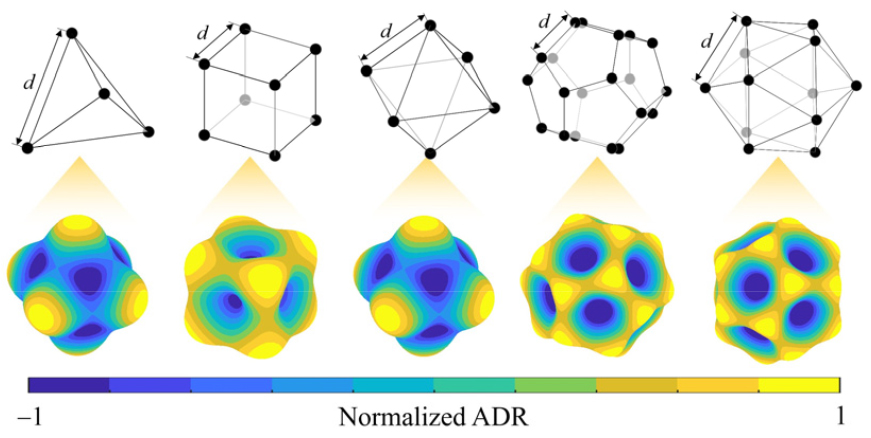
Let Ii (i = 1, 2, … , N) be the intensity vectors estimated from N elemental polyhedral arrays with distinct directional characteristics. Then, the combined intensity vector I+, calculated by their linear combination, is expressed as[12]:
where 𝛾i is a correction constant defined as a function of the Helmholtz number. Because Eq. (4) is derived in terms of Helmholtz numbers, it can be efficiently used, as it allows for the adaptive application of weights corresponding to the hydrophone spacing d and wave number k.
III. Combined hydrophone array
In this study, a 5 channel hydrophone array combining the geometric characteristics of a tetrahedron and a hexahedron was implemented, and its configuration is illustrated in Fig. 2(a). The tetrahedral array performs source localization using hydrophones 1, 2, 3, and 4, whereas the hexahedral array performs localization using hydrophones 2, 3, 4, and 5. Although the hexahedral array takes a truncated form rather than a complete hexahedron, it is isomorphic when transformed into a concentric configuration.[11] Consequently, the identical ADR can be achieved with only four hydrophones, facilitating system implementation with a minimal number of sensors. For simplicity, the tetrahedral array and the hexahedral array are hereafter referred to as Array I and Array II, respectively.
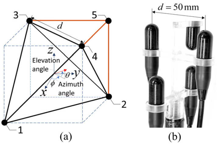
The combined array is formulated by integrating Array I and Array II, which satisfy geometric conditions that mutually compensate for the spatial irregularity of the ADR. This combination is implemented through Eq. (4). Because 𝛾i is a correction constant defined as a function of the Helmholtz numbers, frequency compensated source localization results can be calculated based on the filter designed in a previous study.[12]
Fig. 3 and Table 1 present the simulation results for the source localization, where the sensor spacing is set to d = 50 mm. These results show the DoA estimation performance for sound sources incident from 100 random directions. The test signal was band-limited white noise from 4.8 kHz to 14.9 kHz, corresponding to 1 < kd < π. Overall, the estimation error tends to increase at higher measurement frequencies; however, one can see that the combined array demonstrates a relatively lower estimation error compared to Array I and Array II.
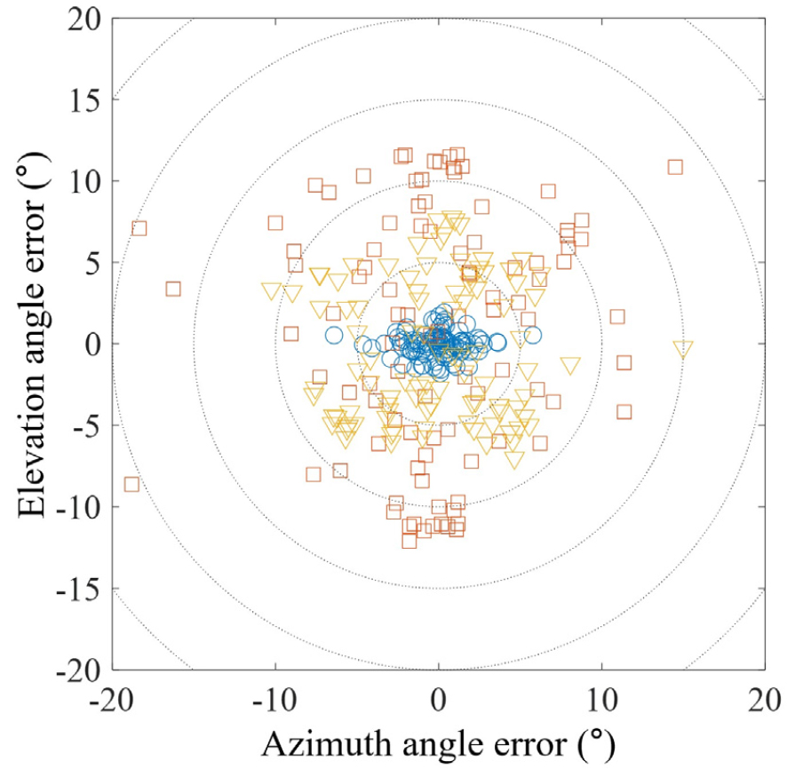
 , Array I;(
 , Array II; (
 , combined array.
Table 1.
Simulation results.
| Array I | Array II | Combined array | ||||
| mean | s.d. | mean | s.d. | mean | s.d. | |
| 1 < kd < 2 | 2.6° | 0.8° | 1.5° | 0.4° | 0.9° | 0.1° |
| 2 < kd < π | 7.6° | 3.2° | 4.8° | 2.0° | 1.2° | 0.5° |
A hydrophone array was implemented that has low error at high Helmholtz numbers, as shown in Fig. 2(b). Using the combined hydrophone array, this study experimentally validated a sound source localization system to demonstrate the localization performance in the frequency domain.
IV. Phase calibration
In sound source localization, calculations are fundamentally based on the phase differences of the sound pressures reaching the sensors; therefore, compensating for inherent phase mismatch is crucial. To this end, phase calibration is required, and a calibration system was designed as shown in Fig. 4.
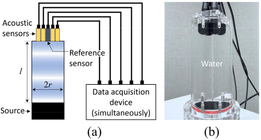
Here, a piezoelectric sensor with an internal amplifier, specifically an Integrated Electronics Piezo Electric (IEPE) type, is used as the hydrophone to construct the array, and the system is designed to calibrate the hydrophones simultaneously. An acoustic source (H1a, Aquarian Audio & Scientific) with a flat, acoustically transparent adaptor was attached to one end to generate a plane wave within the cylinder with a radius of r = 0.02 m and l = 0.12 m.
This setup enables phase calibration over a frequency band up to 21 kHz, a cutoff frequency corresponding to kr < 1.84, which is strictly before emerging the first circumferential mode. Furthermore, the distance l between the source and the measurement plane was determined to satisfy the far-field condition at the sensor locations by considering kl > 1. Considering the dimensions of the hydrophone to be calibrated and the cylinder size, up to four hydrophones can be calibrated simultaneously, with a minimum spacing of 14 mm between adjacent sensors. Since five hydrophones were used in this study, a total of four sets of calibrations were performed based on a reference. For each set, spatial averaging was conducted at 90° intervals around the cylinder axis.
Data acquisition devices (9234, National Instruments), a power amplifier (2719, Brüel & Kjær), and a function generator (33500B, Keysight) were used for the experiment at a sampling rate of 51.2 kHz. Pure water at approximately 24.5 °C was used as the medium; the corresponding speed of sound is 1495 m/s.[13]
Fig. 5 shows the inherent phase mismatches calculated through the phase calibration of the five hydrophones. A sine sweep signal ranging from 500 Hz to 22 kHz was fed into the source, and the measurement results were averaged over 1/3-octave bands; the results are represented at the center frequencies. Here, Sensor 1 was used as the reference to compare the phase differences of the other sensors. It was observed that Sensor 2 exhibited a distinct phase mismatch compared to the others. Such an inherent phase mismatch makes it difficult to guarantee measurement repeatability, as it may indicate a systematic problem, such as linearity, even after compensation for the phase differences. Because it is desirable to exclude sensors with these anomalies from actual experiments, Sensor 2 was replaced with another hydrophone of the same type.
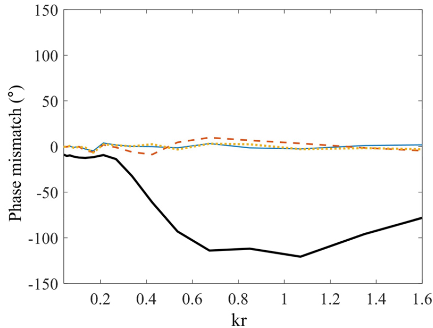
 , Sensor 3:(
 , Sensor 4:(
 , and Sensor 5:(
 are indicated.
V. Experiment
An underwater sound source localization experiment was conducted using the proposed hydrophone array. The experiment was conducted in a 2.6 m × 2.1 m × 2.0 m water tank, and the experimental setup is shown in Fig. 6. The water temperature was 24.5 °C, with a calculated speed of sound of 1495 m/s. Nine 1/3-octave band-limited white noise within the 0.4 < kd < 3.8 range were utilized as sound source signals, with the center frequencies of 2.5 kHz, 3.2 kHz, 4 kHz, 5 kHz, 6.4 kHz, 8 kHz, 10 kHz, 12.7 kHz, and 16 kHz, respectively. The burst signals with a duration of 2 ms and a 1 s interval were repeatedly measured 10 times. The measurement signals were time-gated using a rectangular window of 0.45 ms based on the arrival time of the sound to exclude boundary reflections. And then concatenated the time-gated signals to calculate a CPSD with 10 non overlapping averages using Welch’s method. The acoustic centers of the projector and the hydrophone array were fixed at 1 m from the water surface to hold the reference elevation angle at 0°, which has no spatial bias error in the elevation angle, ideally. The reference DoA of the sound source was controlled by adjusting a rotator mounted on the measurement system, varying the relative azimuth angle between the source and the receiver.
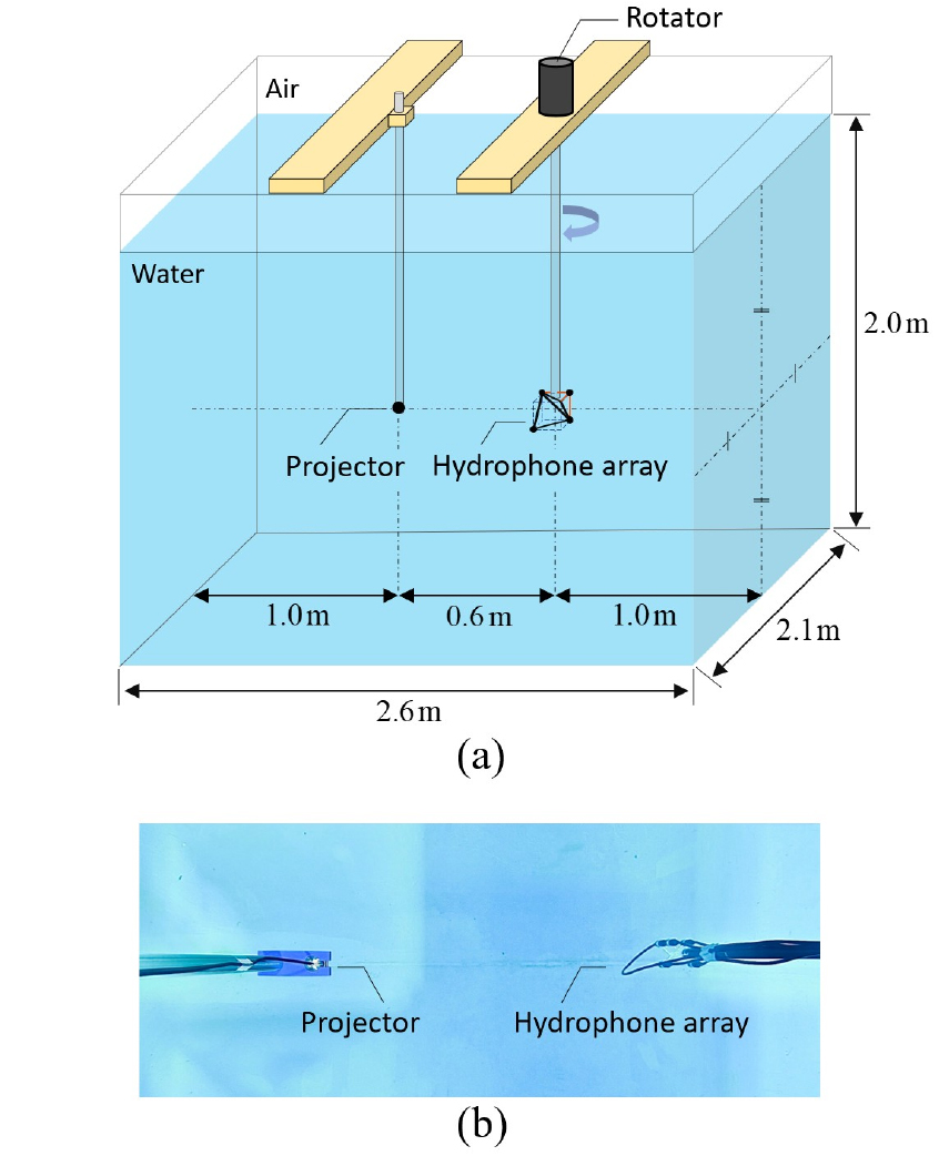
Fig. 7 shows the localization results for reference azimuth angles of 30° and 60°, respectively. One can see that the spatial bias errors of Array I and Array II exhibit opposite trends depending on the reference angles. This is due to the distinct spatial characteristics of the ADR that each array exhibits across varying directions. For kd > 1, as the Helmholtz number increased, the errors in Arrays I and II increased rapidly due to spatial bias, demonstrating bearing angle errors of up to 16° and 12°, respectively.
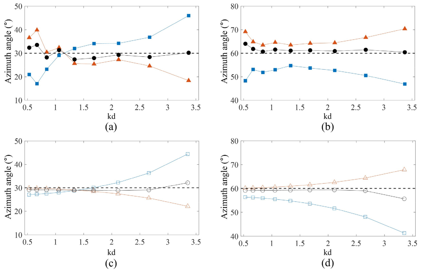
Fig. 7.
(Color available online) (a)(b) Sound source localization test results of the experimental setup, and (c)(d) simulation test results for comparison: (a)(c) reference direction of arrival of sound source is 30°, (b)(d) 60°. Here, (
 ,(
,(
 are the results for Array I; (
 ,(
,(
 Array II; (
 ,(
,(
 combined array; dashed line indicates the actual DoA of the sound source.
In contrast, the combined array has only small bias errors, with localization results showing maximum errors of less than 3° for all Helmholtz numbers. The experimental results show a trend similar to the simulation results indicated in Fig. 7(c) and (d), confirming that the proposed design model operates effectively in the actual underwater environments. However, a tendency for the error to increase slightly was observed in the kd < 1. This is because the valid signal window prior to the arrival of reflected sound is extremely short, i.e., less than 1 ms. In other words, in the low frequencies, the effective time window of the measurement signal was too short relative to the long wavelength, so it is hard to secure a sufficient number of valid wave cycles for calculation. This is a limitation stemming from the experimental environment, and it is expected that this limitation can be resolved by utilizing a larger water tank. In this study, the influence of flow induced noise was excluded by testing in a water tank; however, estimation errors caused by such non acoustical noise may occur in actual application test environments, and further review of this influence is required in future work.
VI. Conclusions
In this study, a 5 channel combined hydrophone array system for sound source localization was proposed and experimentally validated. To overcome the spatial irregularity of the ADR, tetrahedral and hexahedral structures were linearly combined in a concentric configuration. In addition, phase calibration was conducted to compensate for the inherent phase mismatch between the hydrophones to ensure hardware robustness. The experimental results showed that the combined array has accurate localization results across the entire frequency range. This means that the proposed hydrophone array based localization can effectively extend the operational frequency bandwidth in underwater applications with a minimal sensor count. Therefore, it can offer a practical geometric array combination method for high precision underwater surveillance systems.