

I. Introduction
II. System model
III. Proposed ACM mode classifier
3.1 Input parameters for classifier training
3.2 Learning based ACM mode selection
IV. Simulation results
V. Conclusions
I. Introduction
Traditional Underwater Acoustic Communication (UAC) systems are generally use a fixed set of a single modulation and coding scheme. However, since UAC environments exhibit rapidly changing channel characteristics due to factors such as multipath delay spread and Doppler shift, it is challenging to cope with a large variety underwater channel only using fixed scheme. To the end, the Adaptive Coding and Modulation (ACM) schemes which adaptively switching among different modulation and coding scheme according to current channel conditions are essential to achieve high transmission efficiency.[1] However, setting selection criteria for ACM modes, defined by combinations of coding rate and modulation order, is particularly challenging in such environments. This paper analyzes four transmission modes with different data rates and modulation formats. To address the challenge of mode selection under time-varying channel conditions, we propose a Machine Learning (ML) based classifier that predicts the optimal ACM mode by learning from CQI.[2,3] Conventional ACM selection methods rely on static thresholds of Received Signal-to-Noise Ratio (RSNR) or predefined LUT (Look Up Tables).[4] These approaches are unable to adapt to the time-varying nature of underwater acoustic channels. Recently, various ML based ACM prediction methods have been applied to dynamic channel environments. Recent studies have introduced a variety of ML based ACM mode selection methods, including reinforcement learning using CQI and Hybrid Automatic Repeat reQuest (HARQ) feedback via Deep Q-Networks (DQN),[5] Deep Neural Network (DNN) regression models based on Signal-to-Interference-plus-Noise Ratio (SINR) and distance,[6] and random forest classifiers trained on real-world channel measurements.[7] These approaches outperform static table based methods in terms of adaptability and responsiveness to dynamic environments. However, existing methods still have notable limitations. First, many rely solely on prediction accuracy as the evaluation metric, without accounting for actual communication success or effective throughput. Second, regression based approaches that apply thresholds after prediction often misclassify samples near decision boundaries, potentially leading to communication failure. To overcome these limitations, this paper proposes a ML based ACM mode selection strategy that jointly considers both reliability and transmission efficiency.
In this paper, we assume that channel variation between the CQI measurement and the data transmission within a frame is negligible. We applied Estimated Coded Bit Error Rate (EC-BER)[8] for decoding reliability. By training only with samples that meet EC-BER thresholds, the classifier’s performance is improved. The classifier is trained using four CQI including Input SNR (ISNR), RSNR, Pilot-Bit Error Rate (P-BER), and Channel Impulse Response (CIR), each representing a distinct aspect of underwater channel quality. We analyze the effect of EC-BER threshold filtering and demonstrate that this method improves the classification accuracy.
II. System model
The proposed system is designed to select the optimal ACM mode in real time based on CQI in a UAC environment. It consists of two primary components: a transmitter-receiver architecture and a ML based ACM classifier.
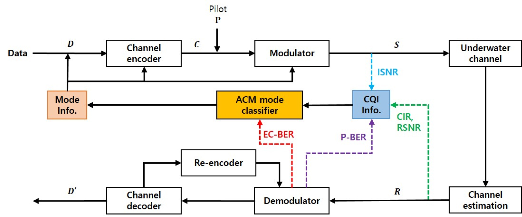
Fig. 1 shows the overall block diagram of ML based ACM system. It consists of two primary components: a transmitter–receiver architecture and ACM classifier. The proposed system is designed to select the optimal ACM mode in real time based on CQI in a UAC environment. At the transmitter, a bitstream of length is encoded using a turbo encoder, generating a coded bit sequence . A pilot sequence of length is inserted, resulting in a total of bits. These bits are modulated to form the transmitted signal , where is the number of modulation symbols. The received signal at the receiver is expressed in Eq. (1) as:
Where:
: Number of multipath components,
: Channel coefficient for the l-th path,
: Additive white Gaussian noise (AWGN).
To enable ACM mode selection, the packet is structured in two formats, as shown in Fig. 2. Fig. 2(a) shows the initial pre-transmission packet, which contains a Linear Frequency Modulated (LFM) signal and a pilot signal.[9] This packet is used solely for channel estimation, without transmitting any data. Fig. 2(b) shows the ACM data packet, which consists of an LFM preamble, a mode index, 200 pilot symbols, and 600 data symbols. The mode index serves as a unique identifier of the ACM mode selected at the transmitter, enabling the receiver to perform demodulation and decoding according to the selected mode.
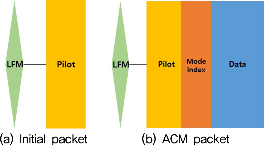
With a sampling frequency of 192 kHz and 96 samples per symbol(), the symbol rate is 2 ksps. The LFM signal serves for synchronization and indicates the modulation type: up-chirp represents to QPSK(Quadrature Phase Shift Keying) and down-chirp represents to BPSK(Binary PSK). Based on this structure, the receiver estimates CIR, RSNR, and P-BER from the pilot. The transmitter then selects the appropriate ACM mode and transmits the data accordingly. Table 1 shows the four ACM mode configurations. Each mode varies in input data size, modulation, and coding rate. We consider QPSK and BPSK modulation and turbo codes with coding rates of 1/2 and 1/3. Without loss of generality in analyzing performance, all modes have same length of pilot and modulated data symbols. The proposed ML-based ACM classifier is located at the transmitter, as shown in Fig. 1, since the transmitter must determine the coding and modulation schemes before data transmission. The receiver estimates the CQI from the pilot symbols, and then feeds them back to the transmitter. Based on feedback information, ML- based ACM classifier determine which mode is optimal in current underwater environments.
Table 1.
ACM mode configurations.
ML-based ACM classifier is carried out using a random forest classifier. This ensemble learning method constructs multiple decision trees using a bootstrap aggregation strategy.[10] The selection of the optimal transmission mode is carried out using a random forest classifier. It is characterized by fast training and strong resistance to overfitting, which makes it particularly suitable for the proposed method. This is because the classification task in proposed system involves input features (ISNR, RSNR, P-BER, CIR) with non-linear relationships to the optimal ACM mode. Random forest can effectively handle such diverse features without requiring feature normalization, and its ensemble structure ensures stable performance even with a limited training dataset. Moreover, the feature importance analysis provided by random forest allows intuitive interpretation of which CQI metrics most influence the ACM decision.
III. Proposed ACM mode classifier
3.1 Input parameters for classifier training
Due to the highly time-varying and complex nature of underwater channels, an adaptive mechanism for selecting suitable ACM modes becomes indispensable. Therefore, this study proposes a ML based classifier that selects the optimal ACM mode using the following four key input parameters:
- ISNR (Input Signal-to-Noise Ratio)
- RSNR (Received SNR)
- P-BER (Pilot Bit Error Rate)
- CIR (Channel Impulse Response)
ISNR is defined as the baseline symbol energy–to–noise density ratio (). We normalize the symbol energy to =1 and use samples per symbol. AWGN is then added after the multipath filtering with its per–sample variance calibrated so that the average SNR per symbol equals the target ISNR. It is defined in Eq. (2) as:
Where, denotes the variance of the zero-mean Gaussian noise samples added to each received sample.
RSNR is estimated using known pilot signal exchanged between the transmitter and receiver. It is defined in Eq. (3) as:
Where, denotes the received pilot signal, the segment of in Eq. (1) corresponding to the pilot symbols, and denotes the corresponding ideal transmitted pilot signal. is the average power of the transmitted pilot symbols, while represents the mean squared error between the received and the ideal pilot signals. Prior to computing RSNR, we estimate a pilot-based complex gain and normalize the received pilot to the reference . A higher RSNR indicates that the received pilot more closely matches the ideal pilot, reflecting more accurate channel estimation and thus improved decoding performance.[11]
P-BER is calculated from the demodulated pilot signal and serves as an indirect indicator of synchronization accuracy and channel estimation quality.[12] Because pilot signal are transmitted without coding and undergo the same channel impairments as the data payload, P-BER is highly correlated with the data error rate. According to References [13, 14], when employing a turbo code with a 1/2 coding rate, reliable decoding is generally achievable when P-BER is below 10 %. Conversely, a P-BER exceeding this threshold leads to a significant degradation in decoding performance and a higher likelihood of data errors. CIR characterizes the time-domain response of the underwater channel and includes important attributes such as the number of multipath components, path delays, and attenuation.[15] To illustrate the scenario considered in this paper, we use three example CIRs (Fig. 3) with a transmitter–receiver separation of 1 km.
-CIR 1: Ideal single-path scenario with no multipath.
-CIR 2: Moderate multipath scenario with two paths (delay = 5 ms, attenuation = 0.8).
-CIR 3: Severe multipath scenario with three paths (delay = 5 ms, 10 ms; attenuation = 0.8, 0.6).

These four parameters are all measurable in real time, and these effectively reflect the current channel condition and possiblity of successful communication. Therefore, they are used as input features to train the ACM classifier.
In the simulation, four ACM modes (Mode 1 ~ 4) were evaluated under three multipath channel scenarios(CIR 1 ~ 3) across an input SNR range from –25 dB to 20 dB with 0.5 dB increments. For each channel condition, 10,000 independent packet transmissions were simulated, resulting in a dataset of approximately 10.9 million labeled samples. Among them, 70 % were used for training, 15 % for validation, and 15 % for testing. Each sample consisted of four CQI(ISNR, RSNR, P-BER, CIR) as input features and the optimal ACM mode as the label determined by the performance score criterion.
3.2 Learning based ACM mode selection
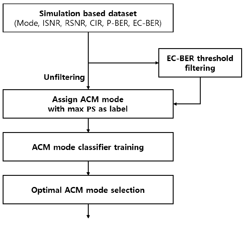
Conventional ACM selection methods typically rely on fixed RSNR thresholds or predefined lookup tables. A LUT (Look Up Table)-based ACM method is simple and practical when only a few CQI with fixed thresholds are used, but it faces structural limitations as CQI (e.g., Doppler, multipath) increase tables and decision boundaries remain discontinuous. We propose a method that learns from LUT-derived labels on the same dataset under identical EC-BER filtering, reproducing LUT performance while providing continuous decision boundaries and natural extensibility to higher-dimensional CQI. The proposed method assumes negligible channel variation between CQI estimation and data transmission. Fig. 4 shows the label generation and classifier training process for ACM mode selection. The overall process includes the following five steps:
Step 1: Data Collection: A simulation based dataset is built, containing various SNR levels and combinations of the three CIRs for each ACM mode. For each transmission, CQIs such as ISNR, RSNR, CIR, P-BER, and EC-BER are collected. EC-BER evaluates the accuracy of the decoding process.
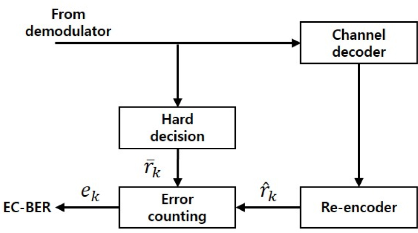
Step 2: The EC-BER is used to evaluate the reliability of received data by comparing the re-encoded bits with the hard-decision output from the demodulator.
As illustrated in Fig. 5, EC-BER measures the number of mismatches between the hard-decoded symbols and the corresponding re-encoded bits . The procedure for error counting is defined in Eqs. (4) and (5).
Where is the index of error for the -th bit, and EC-BER is computed as the percentage of bit mismatches between the re-encoded output and the demodulated input over N bits. Thus, EC-BER has a close relationship with the decoding performance. A small number of input errors to the decoder leads to a low EC-BER, indicating reliable decoding performance.
Step 3: Data Filtering: Only samples satisfying EC- BER thresholds are retained: ≤ 10 % for coding rate 1/2 and ≤ 15 % for 1/3. This ensures that only decodable cases are used for training.
To validate the effectiveness of EC-BER filtering, Fig. 6 compares EC-BER and actual Decoded BER (D-BER) under the ideal CIR 1 scenario. The results show that when EC-BER is below the threshold, D-BER remains within the Quasi Error-Free (QEF) region, confirming successful decoding.[16] To determine appropriate EC- BER thresholds, we analyze the minimum ISNR values required for each mode to enter the QEF region and report the corresponding average EC-BER values in Table 2.
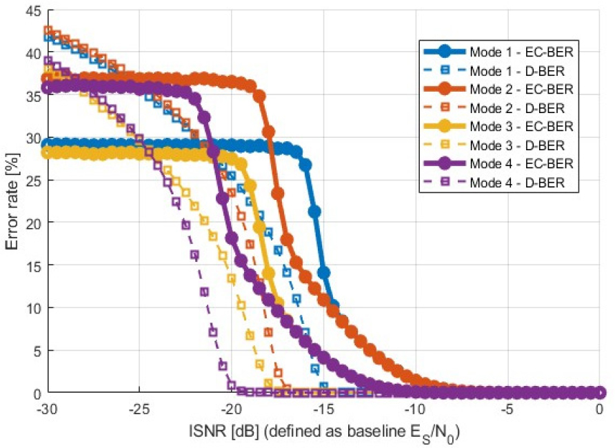
Table 2.
Minimum ISNR and average EC-BER in the QEF region.
| Mode | ISNR (dB) | Average EC-BER ( %) |
| 1 | -14.5 | 10.19 |
| 2 | -17.0 | 17.98 |
| 3 | -17.5 | 10.50 |
| 4 | -19.5 | 15.51 |
Modes 1 and 3, which use a coding rate of 1/2, are considered reliable when EC-BER is ≤10 %. Modes 2 and 4, with a coding rate of 1/3, are acceptable up to an EC-BER of 15 %. These thresholds reflect practical limits for maintaining communication reliability and are used to filter the training dataset.
Step 4: Label Assignment: For each channel sample, among the candidate ACM modes that satisfy the EC-BER threshold, the one with the highest performance score (PS) is selected as the label. The PS is defined in Eq. (6) as:
This step involves selecting the ACM mode with the highest PS among the candidates that satisfy the EC-BER threshold. The performance score jointly reflects decoding success (low EC-BER) and transmission efficiency (high TR), guiding the classifier to learn the best trade-off under each channel condition.
Step 5: Classifier Training and Inference: A random forest classifier is trained using ISNR, RSNR, P-BER, and CIR as input features to learn the optimal ACM mode for each channel condition. Once trained, the classifier predicts the most suitable mode for new channel conditions in real time.
IV. Simulation results
To evaluate the performance of the proposed ML based ACM classifier, extensive simulations were conducted under various underwater channel conditions. The simulations considered four ACM modes across multiple SNR ranges and three CIR profiles. For each simulation, the following CQI were collected: ISNR, RSNR, P-BER, CIR, and EC-BER. After data collection, only valid transmission cases that satisfied the EC-BER thresholds were filtered and used to label the dataset. The ACM mode with the highest PS under each condition was selected as the ground truth label, and a random forest classifier was trained accordingly. In this section, we analyze and compare the performance of two classifiers:
-Unfiltered Training Classifier: Trained on all received data, regardless of EC-BER.
-Filtered Training Classifier: Trained only on data that satisfy the EC-BER threshold.
Fig. 7 shows the feature importance values for both classifiers, as calculated by the random forest algorithm based on the Gini importance criterion. P-BER was consistently ranked as the most important feature, indicating its strong influence on ACM mode prediction. This aligns with the fact that pilot demodulation accuracy is closely correlated with decoding reliability. RSNR and ISNR also demonstrated high importance, reflecting their contribution to overall signal quality. In contrast, CIR showed relatively lower importance, despite containing multipath information. This may be due to its indirect contribution, as its impact is already reflected in P-BER and RSNR.
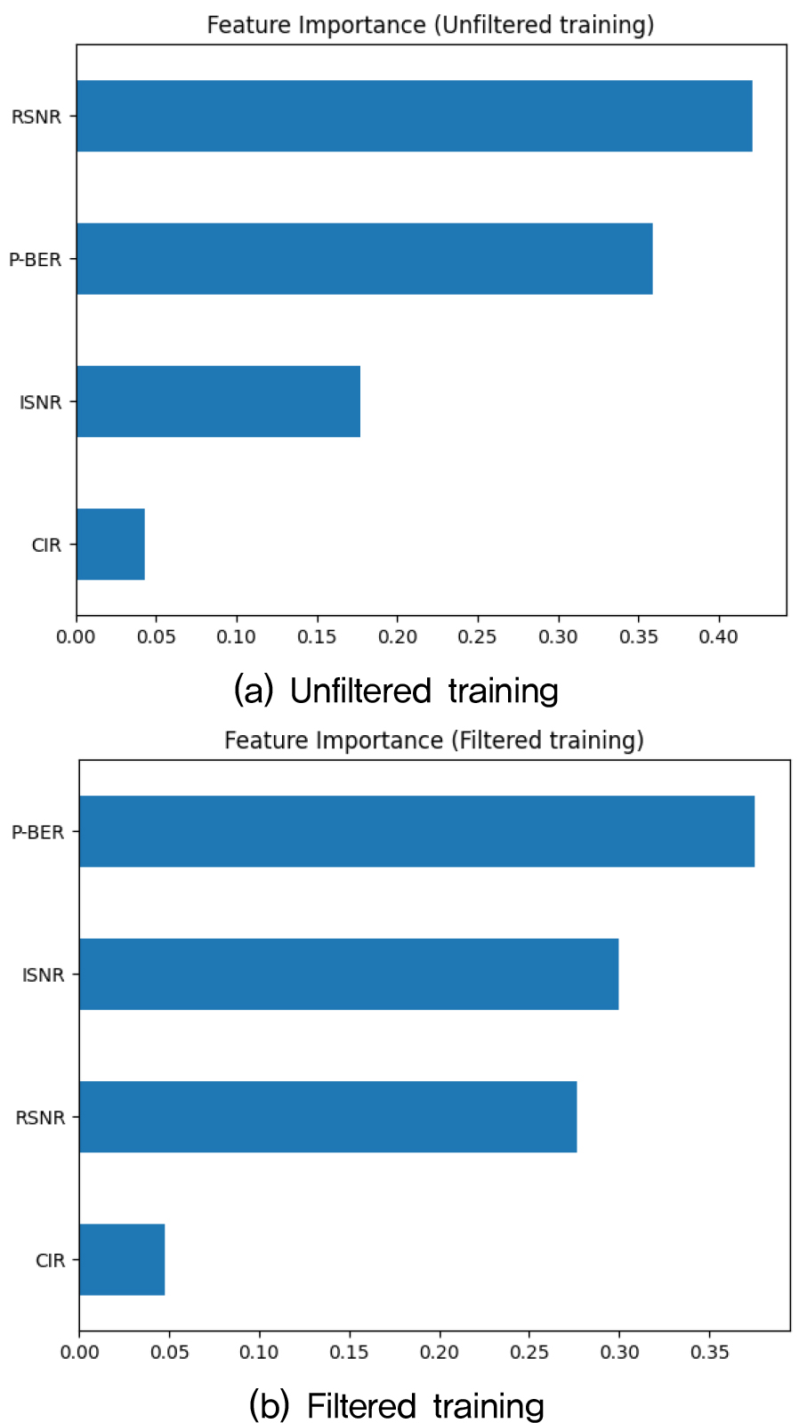
For the filtered-training classifier, we conducted a Monte Carlo–based sensitivity analysis of the four input features (ISNR, RSNR, P-BER, and CIR). We applied additive Gaussian noise (𝜎 = 0.5 dB) to ISNR and RSNR, and modeled the measurement variability of P-BER with a binomial variance determined by the pilot-bit length. Single-feature sensitivity analysis shows contributions of 30.3 % (P-BER), 19.5 % (RSNR), 13.8 % (ISNR), and 0.8 % (CIR), indicating that P-BER and the SNR features are the primary determinants of ACM mode selection. Thus, P-BER’s elevated sensitivity mainly reflects statistical variability due to the finite number of pilot bits.
Fig. 8 shows the confusion matrix to evaluate the classification performance of the proposed ACM mode selection system. Each row corresponds to the actual label, and each column indicates the predicted label. In Fig. 8(a), the classifier trained without EC-BER filtering shows generally high accuracy, but some misclassifications are observed, particularly in specific modes. In contrast, Fig. 8(b) shows that the classifier trained with filtered data produces more accurate predictions especially for Modes 2 and 4. which had shown relatively lower prediction accuracy in the unfiltered case.
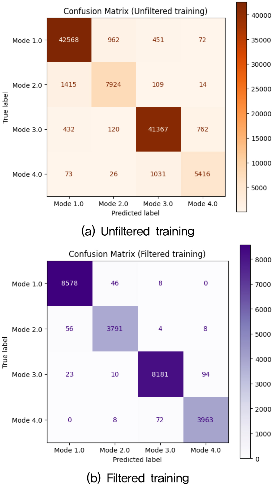
This improvement is attributed to the fact that training was conducted only on valid data satisfying the EC-BER threshold, which leads to more distinct class boundaries and improves the overall stability of the classification model. Moreover, as shown in Fig. 8(b), it can be observed that Modes 2 and 4 appear less frequently compared to Modes 1 and 3, indicating a class imbalance among ACM modes. This imbalance arises from the labeling strategy, which prioritizes the highest transmission rate among valid modes that satisfy the EC-BER threshold.
To quantitatively compare the classification results, Table 3 presents evaluation metrics including accuracy, precision, recall, and F1-score, calculated for each ACM mode. Accuracy indicates how many predictions were correct out of the total. Precision reflects how many of the predicted instances for a given class were actually correct, while recall shows how many actual instances of that class were successfully identified. F1-score is the harmonic mean of precision and recall.
Table 3.
ACM mode performance indicators depending on data filtering.
As shown in Table 3, the unfiltered training classifier achieved an overall accuracy of 94.68 %, with average precision and recall around 0.94 across modes. In contrast, the filtered training classifier achieved significantly improved results, with precision, recall, and F1-score exceeding 0.98 for all modes and an overall accuracy of 98.70 %. These results indicate that training with filtered data, which includes only reliably decodable samples, improves both the generalization ability and stability of the classifier. In particular, the filtered model more clearly distinguishes between similar modes. This reduces ambiguity near decision boundaries and enables the classifier to learn data-driven mode separation, rather than relying on fixed thresholds. The results clearly demonstrate that using only reliable, EC-BER-qualified data enhances the classifier’s generalization capability and decision accuracy.
Fig. 9 compares the EC-BER performance of fixed transmission modes and the proposed classifier based ACM system under identical channel conditions. Each marker represents the EC-BER result of either a fixed mode or the mode selected by the classifier. In low ISNR regions, the classifier tends to select lower-rate modes (e.g., Mode 4), while in high ISNR regions, it selects higher-rate modes (e.g., Mode 1). This adaptive selection enables stable EC-BER performance to be maintained across the entire ISNR range.
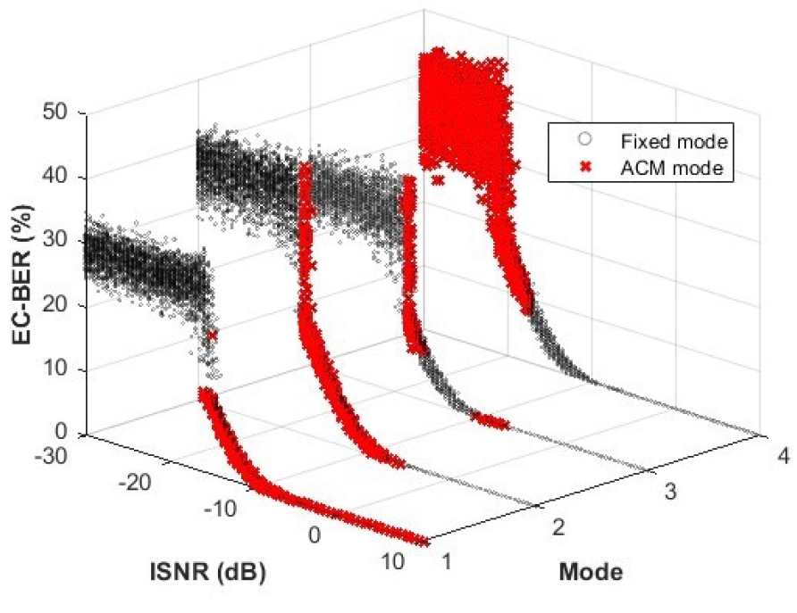
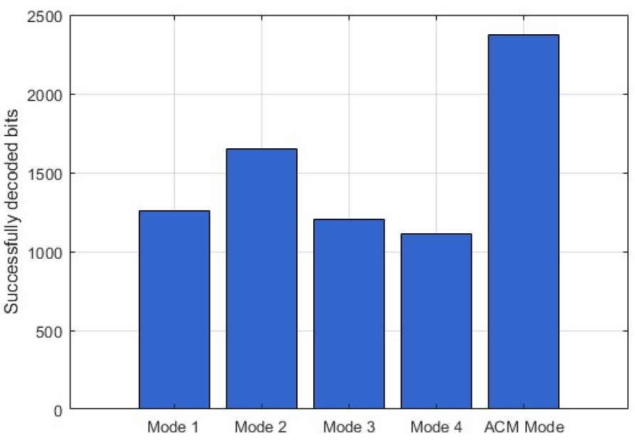
Fig. 10 shows the cumulative number of successfully decoded bits for each mode under varying channel conditions. The classifier based ACM system outperforms all fixed transmission modes in terms of overall throughput. Specifically, it achieves approximately 1.5 times higher throughput than the best-performing fixed mode (Mode 2), and nearly twice as much as the lowest-performing mode (Mode 4). These results confirm that the proposed ML based ACM mode selection method significantly improves both reliability and transmission efficiency across diverse underwater channel environments.
V. Conclusions
This paper proposed a ML based ACM mode selection method for UAC systems operating in highly time-varying channel environments. The method utilizes four CQI (ISNR, RSNR, P-BER, and CIR), as input features to predict the optimal ACM mode under given channel conditions. The classifier was trained using only the samples that met predefined EC-BER thresholds, ensuring that the training data consisted of reliably decodable transmissions. A random forest classifier was used CQI values to switch optimal ACM mode, based on a performance score that considers both decoding reliability and transmission efficiency. The classifier trained with EC-BER-filtered data achieved an accuracy of 98.7 percent. In simulation results, the proposed method achieved approximately from 1.5 times to 2 times higher throughput compared to fixed mode method, while satisfying QEF range of decoding performance. Therefore, the proposed method demonstrates strong adaptability and performance under diverse underwater conditions and offers a practical solution for dynamic link adaptation. Future research will include expanding the dataset using real-world measurement data, addressing class imbalance in training, and incorporating additional channel parameters such as Doppler spread and time dispersion into the learning model.
