I. 서 론
배열 센서를 이용한 음원의 위치 추정은 레이더, 소나, 통신 등 다양한 분야에서 중요한 문제이다.[1-9] 초기 다양한 위치 추정기법들은 대부분 원거리(far field) 음원을 가정하였다. 원거리 음원일 경우 센서에 도달한 음파를 평면파로 가정하여 음원의 위치는 방위각에 의해 결정된다. 그러나 음원이 근거리에 위치하는 경우 음파를 구형파로 모델링해야 되며 음원의 위치 추정은 방위각과 거리 추정이 함께 이루어져야한다.
최근 선형 선배열에서 근거리 위치 추정에 관한 연구가 많이 진행되었다.[3-8] 그중 가장 일반적인 기법으로는 1차원 탐색 기법을 2차원으로 확장한 ML,[3] 2차원 MUSIC[4] 기법이 있으나 연산량이 많이 필요한 단점이 있다. 2차원 탐색을 피하기 위해 선형 예측 기법(linear prediction),[5] higher-order ESPRIT,[6] cumulant 기반[7]등의 기법이 제안되었지만 추가적으로parameter pairing이 필요하거나 고차 통계량을 이용한다. 또 다른 기법으로 대칭 선배열에서 거리와 방위를 분리하여 1차원 탐색으로 위치를 추정하는 기법이 제안되었으나 역시 두 단계의 탐색과정이 필요하다.[8]
본 논문에서는 근거리 음원의 위치 추정에 필요한 연산량을 줄이기 위해 선형 배열의 대칭성과 MP기법을 이용하여 탐색과정 없이 방위를 추정하는 기법을 제안한다. 거리 추정은 추정된 방위 값을 이용하여 1차원 MUSIC 기법을 이용한다.
II. 신호 모델
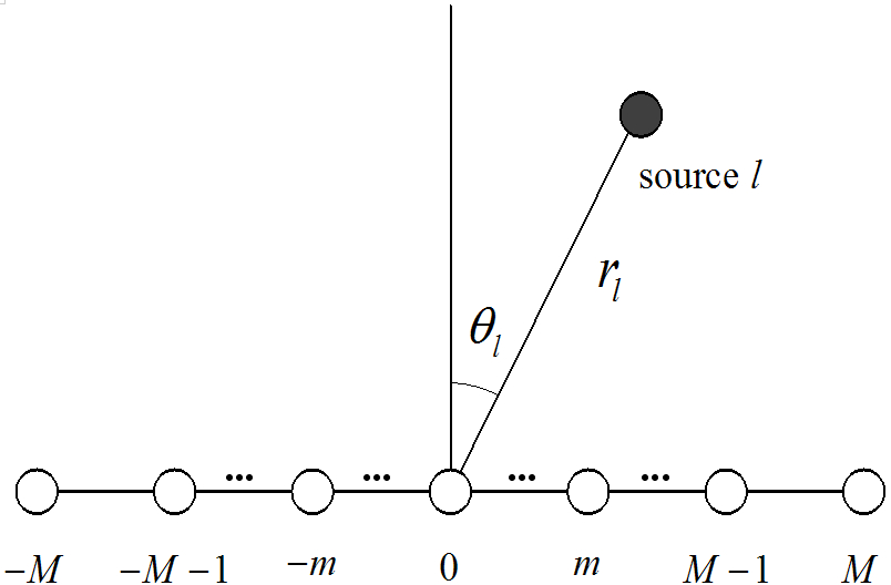
Fig. 1은 가운데 센서를 기준으로 ![]() 개의 센서로 이루어진 선배열의 기하학적 구조이다.
개의 센서로 이루어진 선배열의 기하학적 구조이다. ![]() 개의 음원이 근거리에서 선형 선배열에 입사 되며 각 센서는 위상의 모호성(ambiguity)이 발생하는 것을 피하기 위해
개의 음원이 근거리에서 선형 선배열에 입사 되며 각 센서는 위상의 모호성(ambiguity)이 발생하는 것을 피하기 위해 ![]() 축을 따라
축을 따라 ![]() 간격으로 배치되어 있다. 이때
간격으로 배치되어 있다. 이때 ![]() 는 수신 신호의 파장을 나타낸다. 가운데 센서를 위상의 기준점으로 가정하였을 때
는 수신 신호의 파장을 나타낸다. 가운데 센서를 위상의 기준점으로 가정하였을 때 ![]() 번째 센서에 수신된 신호는 식(1)로 나타난다.
번째 센서에 수신된 신호는 식(1)로 나타난다.
|
Fig. 1. Geometry of uniform linear array and source. |
| (1) |
여기서 ![]() 은
은 ![]() 번째 음원 신호로 센서 간 상호 독립을 가정하며,
번째 음원 신호로 센서 간 상호 독립을 가정하며, ![]() 은
은 ![]() 번째 센서에서의 백색 잡음신호이다. 그리고
번째 센서에서의 백색 잡음신호이다. 그리고 ![]() 은 배열의 중심과
은 배열의 중심과 ![]() 번째 센서사이의
번째 센서사이의 ![]() 번째 음원 신호의 시간 지연을 나타내며 식(2)로 나타난다.
번째 음원 신호의 시간 지연을 나타내며 식(2)로 나타난다.
| (2) |
여기서 ![]() 과
과 ![]() 은 각각
은 각각 ![]() 번째 음원의 거리와 방위이다.
번째 음원의 거리와 방위이다.
표적이 Fresnel 영역에 존재하는 경우 ![]() 은 2차 테일러 전개에 의해 다음과 같이 근사적으로 나타낼 수 있다.[8]
은 2차 테일러 전개에 의해 다음과 같이 근사적으로 나타낼 수 있다.[8]
| (3) |
여기서 ![]() 은
은 ![]() 보다 크거나 같은 항으로 근사적으로 무시 될 수 있다. 식(3)을 이용하면 식(1)을 식(4)로 표현 할 수 있다.
보다 크거나 같은 항으로 근사적으로 무시 될 수 있다. 식(3)을 이용하면 식(1)을 식(4)로 표현 할 수 있다.
| (4) |
수신된 신호의 벡터 ![]() 는 식(5)로 나타낼 수 있다.
는 식(5)로 나타낼 수 있다. ![]() 는 전치를 나타낸다.
는 전치를 나타낸다.
| (5) |
여기서 ![]() 는 신호 벡터이며
는 신호 벡터이며 ![]() 잡음 벡터를 나타낸다. 방향행렬
잡음 벡터를 나타낸다. 방향행렬 ![]() 은 식(6)의 조향벡터
은 식(6)의 조향벡터 ![]() 로 구성된다.[8]
로 구성된다.[8]
| (6) |
 .
.III. 제안 기법
3.1 방위각 추정
방위 추정은 선형 선배열에서 기준 센서를 기준으로 신호가 가지는 대칭성을 이용한다. ![]()
![]() 를 정의 하였을 때
를 정의 하였을 때 ![]() 은 식(7)과 같이 방위
은 식(7)과 같이 방위 ![]() 로만 표현되는 성질을 가진다.
로만 표현되는 성질을 가진다.
| (7) |
여기서 ![]() 은
은 ![]() 번째 음원의 파워,
번째 음원의 파워, ![]() 은 잡음의 파워,
은 잡음의 파워, ![]() 을 나타내며
을 나타내며 ![]() 는 Dirac 델타 함수다.
는 Dirac 델타 함수다.
식(7)과 MP기법을 이용하여 방위를 추정하기 위해 다음 식(8)의 ![]() Hankel 행렬을 정의한다.
Hankel 행렬을 정의한다.
| (8) |
여기서 ![]() 는 pencil parameter로 노이즈 필터링을 위해
는 pencil parameter로 노이즈 필터링을 위해 ![]() 의 값을 가져야 효과적이다.[9] 다음과 같이
의 값을 가져야 효과적이다.[9] 다음과 같이 ![]() 크기의 부행렬
크기의 부행렬 ![]() ,
, ![]() 를 정의하면 식(11), 식(12)의 관계를 가진다.
를 정의하면 식(11), 식(12)의 관계를 가진다.
| (9) |
| (10) |
| (11) |
| (12) |
| (13) |
| (14) |
 ,
,
| (15) |
| (16) |
MP기법으로 ![]() 을 구하기 위해 다음 식을 이용한다.
을 구하기 위해 다음 식을 이용한다.
| (17) |
여기서 ![]() 는
는 ![]() 단위행렬이며
단위행렬이며 ![]() 의 랭크(rank)가
의 랭크(rank)가 ![]() 이 되기 위해서는
이 되기 위해서는 ![]() 의 조건을 만족해야 된다. 식(17)에서
의 조건을 만족해야 된다. 식(17)에서 ![]() 을 구하는 문제는 행렬쌍 {
을 구하는 문제는 행렬쌍 {![]() }의 고유값을 구하는 문제와 동일하다.[9] 따라서 식의 해는 식(18)의 고유값이 된다.
}의 고유값을 구하는 문제와 동일하다.[9] 따라서 식의 해는 식(18)의 고유값이 된다.
| (18) |
여기서 ![]() 는 Moore-Penrose pseudo inverse로 식(19)로 정의된다.
는 Moore-Penrose pseudo inverse로 식(19)로 정의된다.
| (19) |
여기서 ![]() 는 conjugate Transpose이다. 음원의 방위각
는 conjugate Transpose이다. 음원의 방위각 ![]() 은 추정된
은 추정된 ![]() 을 이용하여 식(20)로 주어진다.[9]
을 이용하여 식(20)로 주어진다.[9]
| (20) |
신호에 잡음이 있는 경우 특이값 분해(singular value decomposition)를 통해 잡음으로 인한 효과를 줄일 수 있다. 행렬 ![]() 가
가 ![]() 로 분해될 때
로 분해될 때 ![]() 는
는 ![]() 의 특이값을 주대각성분에
의 특이값을 주대각성분에![]() 와 같이 내림차순으로 포함한다. 만약 신호에 잡음이 없다면 처음
와 같이 내림차순으로 포함한다. 만약 신호에 잡음이 없다면 처음 ![]() 개의 특이값만 0이 아니게 되므로 들어온 신호의 개수를 추정하여 행렬
개의 특이값만 0이 아니게 되므로 들어온 신호의 개수를 추정하여 행렬 ![]() 를 신호 공간과 잡음 공간으로 분리한 후 신호 공간에서 방위를 추정하게 된다.[9]
를 신호 공간과 잡음 공간으로 분리한 후 신호 공간에서 방위를 추정하게 된다.[9]
3.2 거리 추정
![]() 번째 음원의 거리
번째 음원의 거리 ![]() 은 추정된
은 추정된 ![]() 을 식(6)의
을 식(6)의 ![]() 에 대입하여 2차원 MUSIC 기법 대신 식(21)와 같이
에 대입하여 2차원 MUSIC 기법 대신 식(21)와 같이 ![]() 번의 1차원 MUSIC 기법으로 구할 수 있다.
번의 1차원 MUSIC 기법으로 구할 수 있다.
| (21) |
여기서 ![]() 는 수신된 신호의 공분산 행렬
는 수신된 신호의 공분산 행렬 ![]() 의 고유값 분해(eigenvalue decomposition)를 통해 구해진 잡음 부공간을 나타낸다.[8]
의 고유값 분해(eigenvalue decomposition)를 통해 구해진 잡음 부공간을 나타낸다.[8]
IV. 모의 실험
4.1 실험 조건
제안한 알고리즘의 성능을 비교, 검증하기 위해 대칭 부배열 기법(symmetric subarray)[8]과 함께 모의 실험을 수행하였다. Fig. 1의 구조에서 ![]() 의 센서를
의 센서를 ![]() 간격으로 배치하고 두 개의 비상관(uncorrelated) 신호와 센서간에 상호독립인 복소 가우시안 확률변수로 잡음을 가정하였다. 두 음원은 동일한 파워를 가지고
간격으로 배치하고 두 개의 비상관(uncorrelated) 신호와 센서간에 상호독립인 복소 가우시안 확률변수로 잡음을 가정하였다. 두 음원은 동일한 파워를 가지고 ![]() 와
와 ![]() 에 있다고 가정하였다. 실험은 512개의 표본을 이용하여 SNR이 0 dB에서 20 dB까지 수행되었으며 500회 몬테카를로 실험을 수행하여 식(20)으로 정의한 RMSE 값으로 나타내었다. 탐색 간격
에 있다고 가정하였다. 실험은 512개의 표본을 이용하여 SNR이 0 dB에서 20 dB까지 수행되었으며 500회 몬테카를로 실험을 수행하여 식(20)으로 정의한 RMSE 값으로 나타내었다. 탐색 간격 ![]() 은 각각 (
은 각각 (![]() )로 설정하였다.
)로 설정하였다.
| (22) |
여기서 ![]() 은 몬테카를로 실험 횟수,
은 몬테카를로 실험 횟수, ![]() 는 추정하고자 하는 실제 값,
는 추정하고자 하는 실제 값, ![]() 은 추정 값을 나타낸다.
은 추정 값을 나타낸다.
4.2 실험 결과
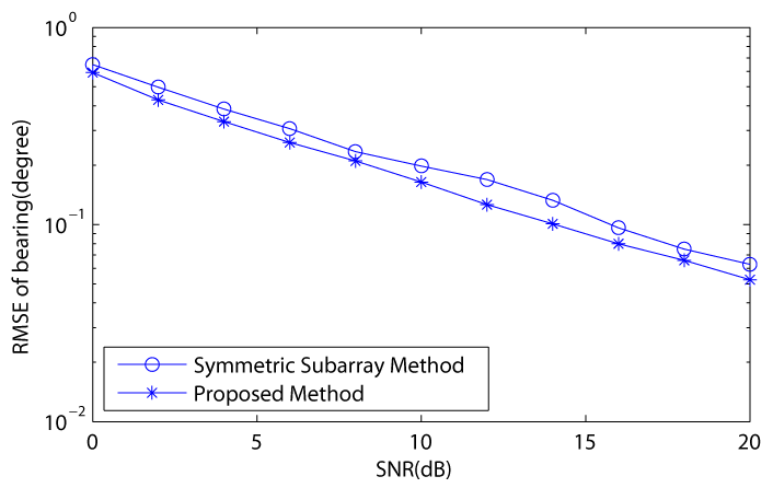
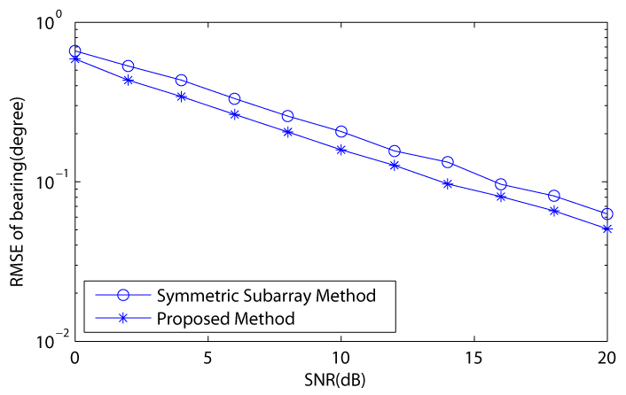
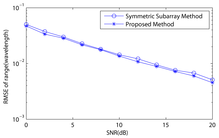
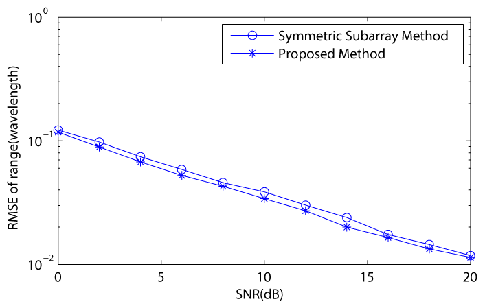
Fig. 2와 Fig. 3은 두 음원의 신호 대 잡음 비에 따른 알고리즘의 위치 추정 성능이다. 실험결과 제안된 알고리즘은 2차원 탐색과정이 필요한 대칭 부배열 기법과 비교하여 다소 우수하거나 유사한 추정성능을 보인다. 연산량 비교를 위해 3.4 GHz 인텔 i7 프로세서에서 MATLAB 프로그램의 ‘tic’, ‘toc’ 명령어로 모의 실험 수행 시간을 측정 하였다. 제안한 알고리즘은 168.62초가 걸린 반면 대칭 부배열 기법을 이용한 기법은 220.55 초가 소요되어 제안한 기법의 연산량 감소 효과를 확인하였다.
|
(a) first source |
|
(b) second source |
Fig. 2. RMSE versus SNR of bearing estimation. |
|
(a) first source |
|
(b) second source |
Fig. 3. RMSE versus SNR of range estimation. |