I. Introduction

Automatic Music Transcription (AMT) is a task that detects and recognizes musical notes events within a given audio recording. While AMT can be applied to a wide range of musical instruments and genres, the piano has emerged as one of the most extensively researched instruments in this field. One of the primary reasons for the popularity of piano transcription in AMT research is the unique characteristics of the instrument itself. Its percussive onset, and stable pitch make it well-suited for automatic transcription tasks. Furthermore, the piano’s popularity as a solo and accompanying instrument in a wide variety of musical genres make it a highly relevant and important focus for AMT research. Additionally, achieving accurate note-level labels is much easier for the piano compared to the other instruments, thanks to the computer-controlled piano.

Before the recent advances of deep learning, many AMT models used traditional machine learning methodology, such as non-negative matrix factorization,^[1] and hidden Markov model,^[2] or signal processing methods.^[3,4] Then, models using Deep Neural Networks (DNN) outperformed the previous approaches.^[5,6,7] Additionally, the release of a large-scale dataset featuring computer-controlled acoustic piano has significantly contributed to the improved performance of DNN-based AMT models.^[8]

AMT is a versatile task that has numerous potential applications, including music education and analysis. For instance, Kong et al.^[9] demonstrated that using transcribed Musical Instrument Digital Interface (MIDI) as input, rather than raw audio, can improve the accuracy of composer identification models. Additionally, recent research by Zhang et al.^[10] has shown that AMT systems can be utilized to construct MIDI datasets of piano performances, with high levels of transcription accuracy that are suitable for training models in areas such as performer identification or expressive performance modeling.

However, many existing AMT systems are designed for offline scenarios, where the system can process the entire audio input from start to finish. This often results in the use of bi-directional Recurrent Neural Networks (RNNs), which can leverage information from both past and future audio frames to improve note transcription accuracy.^[7,11] However, these approaches are not well-suited to real-time or online scenarios, where it is necessary to transcribe notes in a timely manner, without access to future audio frames.

On the other hand, Kwon et al.^[12] proposed an auto- regressive AMT model, which uses uni-directional RNN and enable on-line transcription without using “future” information. Specifically, the model makes predictions for each audio frame based only on past input audio frames and its own prediction for past input, making it well-suited for real-time applications. Our previous work^[13] implemented a real-time AMT system based on this auto- regressive AMT model. Nevertheless, the system directly employed the model without modifying its architecture or hyperparameters to optimize for real-time performance.

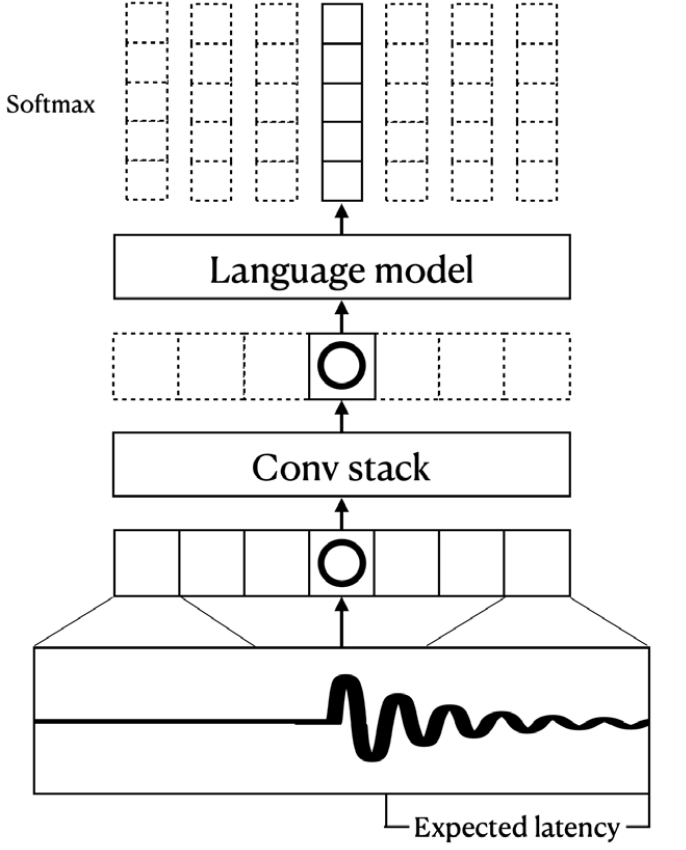
We found that simply using the model as is, without modification, led to certain limitations in terms of the system’s overall latency. This is because the model was not specifically designed to consider the latency of the transcription process, and therefore may require a certain amount of time after a note onset event in order to fully fill the receptive field of the backbone Convolutional Neural Network (CNN) with sufficient audio information. While the computation for each frame of 32 ms can be done in around 12 ms using only a consumer-level Central Processing Unit (CPU),^[13] this intrinsic latency was about 160 ms in the previous work’s setting, as presented in Fig. 1. This clearly exceeds the acceptable range for an interactive application such as real-time remote ensemble, which is known for having tolerance of 100 ms in case of piano.^[14] If an AMT system can achieve latency that is acceptable for ensemble performance, which demands musically coherent synchronization, it will be possible to be employed to various interactive scenarios like piano education or human-machine ensemble.

Fig. 1.

Intrinsic latency is decided by the receptive field of CNN stack.

To address this issue, we explore several different methods for reducing the intrinsic latency of the neural AMT model, with the goal of improving its suitability for a range of interactive scenarios. Through experiments, we demonstrate the effectiveness of these approaches and highlight the potential applications of our optimized neural AMT model.

II. Related work

One of the early full adaptations of deep neural networks for piano music transcription was proposed by Sigtia et al.^[5] This work was the first to propose employing convolutional neural networks as an acoustic model for AMT, and demonstrated that it can outperform previous approaches. Also, the authors propose a hash beam search algorithm to improve inference run times, mentioning its suitability for real-time applications. However, the paper did not introduce an actual implementation of real-time transcription system.

Hawthorne et al.^[7] introduced a significant advancement in neural AMT by proposing dual objective training, which separately predicts onsets and frames. Explicitly training the model to predict onsets led to a notable improvement in transcription accuracy for note onset. The overall structure of using a CNN stack and RNN on top of it was widely adopted in subsequent works.^[11,12,15] Kong et al.^[11] presented a new training objective of regressing onset timing instead of making frame-wise predictions, resulting in a model that outperformed^[7] in most metrics. However, these models are primarily designed for offline scenarios using a bi-directional Gated Recurrent Unit (GRU) on top of CNN stacks.

Several research works have aimed to achieve real-time piano transcription. Akbari and Cheng^[16] proposed a system that uses computer vision to transcribe notes from videos of piano performances, without relying on any audio inputs. Although the system demonstrates high accuracy with low latency, it requires a top-view camera recording of the piano performance, which limits its practical applicability. Additionally, the computer vision approach may not be suitable for other musical instruments beyond keyboards.

Dessein et al.^[17] presented a Non-negative Matrix Factorization (NMF) based model for real-time piano transcription using audio input. This model is designed to learn spectral templates for each individual piano pitch using isolated note samples. During inference, the model fixes the learned spectral templates and decomposes each input spectrogram frame using these templates. The primary advantage of this system is its ability to achieve low latency by making independent inferences for each time frame of the input spectrogram. This allows the system to transcribe the input audio in real-time with minimal latency. However, this approach also has a drawback in that it sacrifices transcription accuracy in favor of speed. By treating each time frame independently and using fixed spectral templates, the system is not able to exploit the information in the temporal progress of audio input. The reported accuracy on MIDI Aligned Piano Sounds (MAPS) dataset^[3] has large gap compared to the deep-learning-based model.^[7]

III. Methods

The latency of CNN-based music transcription model mainly comes from the number of audio samples that the system has to collect more after the onset event happens to feed to the CNN. The CNN layer detects onset-related features when the onset event is placed in its receptive field on the mel spectrogram input. Usually, if the training label and mel spectrogram is aligned in time-frame, the CNN is trained to detect onset when the onset event is located in the center of its receptive field.

Overall, the theoretical expected latency of the CNN can be represented as below,

where r denotes receptive field size of CNN stack in number of time frames of spectrograms, n denotes amount of label shift in terms of frame, and hop and window denote the size of hop and window for spectrogram, respectively. This represents mean latency where the onset event lies in the center of the window, and there is additional ±hop/2 latency based on where the onset lies within the corresponding window.

In this section, we introduce the baseline model^[12] and our modification to reduce the latency.

3.1 Baseline model

We employ an autoregressive multi-state note model^[12] as our baseline model, which is presented in Fig. 2. The model mainly consists of two parts: an acoustic model in CNN and a language model in autoregressive uni- directional Long Short-Term Memory (LSTM). There is a fully-connected layer between CNN and the language model.

Fig. 2.

Architecture of the baseline model.^[12]

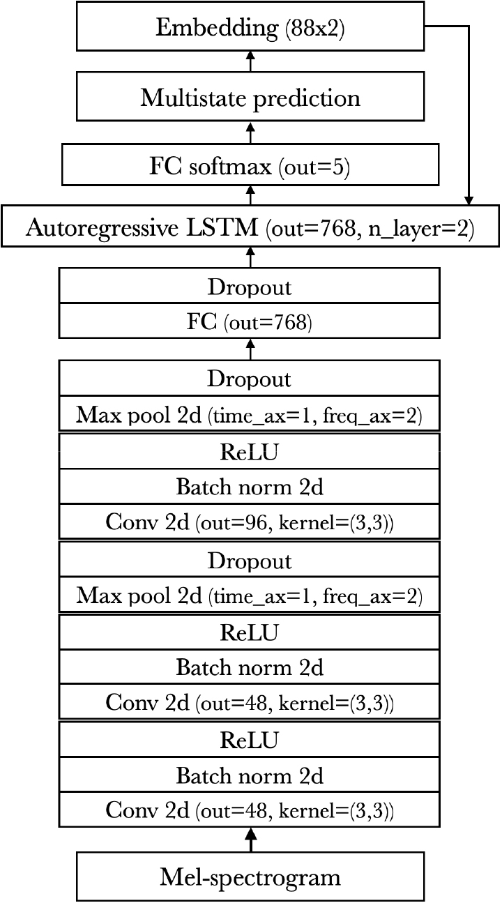
The acoustic model uses a stack of three convolution layers with a kernel size of 3 for both time and frequency axes. The max pooling is done only with the frequency axis, thus preserving the number of time frames throughout the computation. It uses batch normalization after each convolutional layer and Rectified Linear Unit (ReLU) as its activation function.

Throughout the experiment, we only modify the input mel spectrogram or the kernel size of the acoustic model while fixing the fully-connected layer and the language model.

3.1.1 Multi-state note model

One of the widely used framework for solving the music transcription task is to handle it as a multiple binary classification task. For example, Hawthorne et al.,^[7] which first proposed an independent prediction for onset events, calculates losses for onset prediction and frame prediction separately with binary cross entropy loss. Even though the model is designed to consider onset prediction as its input for frame prediction, it is not guaranteed to have a coherent output between the onset predictions and frame predictions. For example, there can be a frame activation without the corresponding onset. On the other hand, the multi-state note model^[12] uses categorical cross entropy. For each pitch for every time step, the label is defined as one of five states, off, onset, sustain, offset, and re-onset. Thus, the ground-truth label for the training can be notated as a I∈{0,1,2,3,4}88×T, where 88 represents number of total pitches in piano, T is a number of time frames, and each integer denotes the corresponding note state class. The details can be found in Reference [12].

3.2 Reducing receptive field size

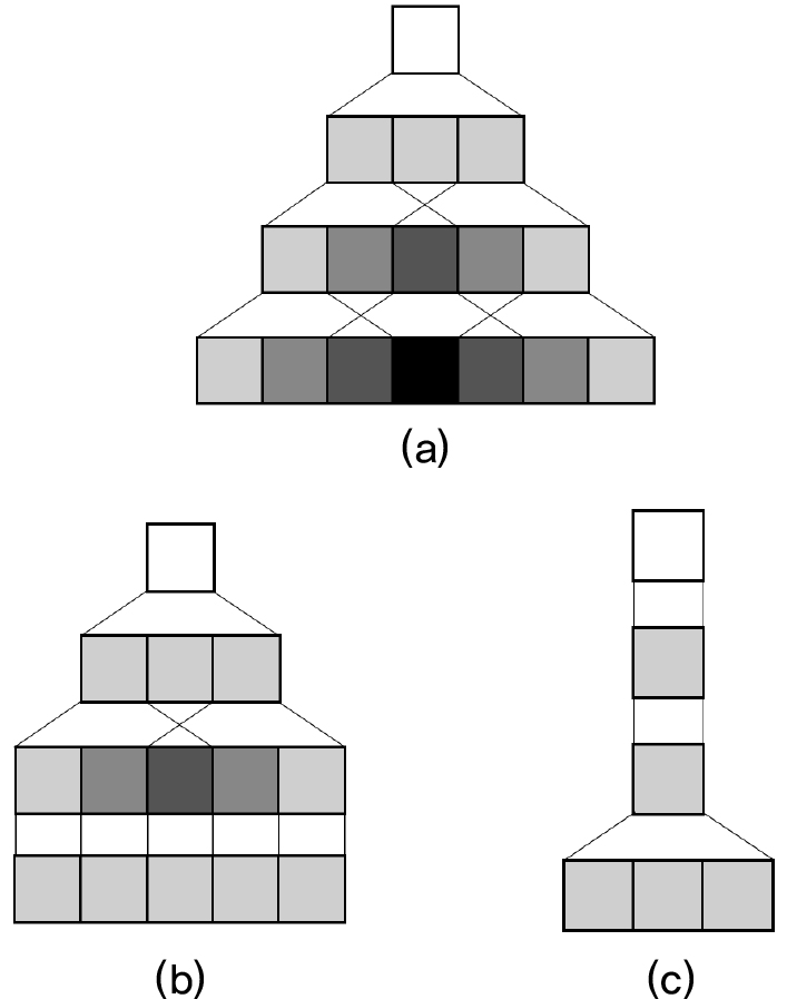
To reduce latency, one approach is to decrease the receptive field of the CNN stack. This can be achieved by reducing the kernel size of a convolution layer from three to one. As a result, the receptive field is reduced for two frames, which is equivalent to a reduction of one time frame in latency. In order to evaluate the trade-offs between latency and transcription performance, we conducted an experiment by varying the kernel sizes.

The baseline model, Kwon et al.,^[12] uses a stack of three convolutional layers with a kernel size of three and padding with one in the time-frame axis. For each of the three layers, we modified the kernel size for the time axis from three to one as presented in Fig. 3, resulting in eight possible combinations. The kernel size for the frequency axis was kept at three for all combinations.

Fig. 3.

Receptive field of CNN stacks with different kernel size. Kernel sizes from input (bottom) to output (top) are: (a) 3, 3, 3 (baseline), (b) 1, 3, 3 (c) 3, 1, 1.

3.3 Shifting label

The current convention in automatic music transcription is to align onset events labels exactly the same with an input spectrogram. This can be represented as an equation below,

where t is onset timing in second, h is a hop length in second, p is a pitch, and ionset is a corresponding index for onset class.

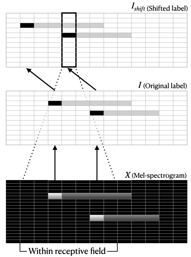
The conventional model uses a convolutional layer with a padding size that preserves the number of time steps, so the output of the CNN for given input X∈ℝF×T is Y∈ℝC×T, where F denotes the number of frequency bin in mel spectrogram and C denotes the number of output channels of the CNN. As the receptive field of the CNN extends in both directions of the time axis, Y[:,t] is calculated using X[:,t-((r-1)/2):t+((r-1)/2)], where r represents the receptive field size of the CNN. If the piano-roll-like label I is aligned with the input mel-spectrogram X, the entire AMT model will be trained to predict the onset event using (r-1)/2 more time frames of mel-spectrogram.

If we shift the label I to n frame earlier so that Ishift[:,:-n]=I[:,n:], the model is forced to use X[:,t-((r-1)/2)-n:t+((r-1)/2)-n] to predict the onset event on t, as presented in Fig. 4. If the shift amount n is less or equal to (r-1)/2, the CNN can be trained to detect the onset since the mel spectrogram frame including the onset event is within the CNN’s receptive field.

Fig. 4.

Shifting label in time axis can enforce the model to detect a note event that occurs in the later part of its receptive field.

3.4 Reducing FFT size of hop size

The latency of the AMT system is also decided by the Fast Fourier Transform (FFT) parameters of the input mel-spectrogram. If we decrease the window or hop size, the latency can be reduced as shown in Eq. (1). Nevertheless, reducing the window size decreases frequency resolution, which can negatively affect transcription accuracy, especially for low-pitched notes. Additionally, using a smaller hop size directly increases the frame rate of the AMT system, requiring more computational resources. In our study, we examined how the accuracy of the model is influenced by using a window size of 1,024 (64 ms) and hop size of 256 (16 ms), which differs from the previous research that used a window size of 2,048 (128 ms) and hop size of 512 (32 ms).^[7,12]

IV. Experiments

4.1 Dataset

For the experiment, we utilized the MIDI and Audio Edited for Synchronous TRacks and Organization (MAESTRO) dataset,^[8] which is the most commonly used dataset for piano music transcription. The dataset comprised of pairs of audio recordings and corresponding MIDI recordings of the piano performance that is captured by a computer-controlled piano, Disklavier. We specifically used v.3.0.0 of the MAESTRO, which omitted chamber music recordings that were erroneously included in v.2.0.0. The total length of audio recordings is 198.7 h, with approximately 7 million notes in total. The dataset also provides predefined train, validation, and test splits, which we adhered to strictly.

4.2 Metrics

The standard metrics for evaluating AMT system are frame-based and note-based F1 score which are provided in mir_eval package.^[18] Note metric evaluates the prediction result decoded as note-level events. Each note event can be represented as a tuple of pitch, onset time, and offset time. Then, we compare the reference notes list and the predicted notes list. As following the convention, a note prediction within 50 ms error is considered as a correct prediction. Since the real-time applications such as ensemble performance or piano education is more sensitive to note onsets rather than frame-wise activation or note offset, we only report precision, recall, and F1 score of note onset metric. The note onset metric was also used for selecting the best training states for each model.

4.3 Training detail

We strictly followed the experiment settings of the previous work,^[12] which was also used in Reference [7], using the PyTorch implementation provided with Reference [15]. For the input, we used log-compressed mel-spectrogram with 229 mel bin, using audio input of sampling rate of 16 kHz. The number of CNN channels and hidden size of LSTM is presented in Fig. 2, which is also the same with Reference [12].

We randomly sliced each data sample into 20 s segments and set the batch size to 16. We used the Adam optimizer with an initial learning rate of 0.0006, which was multiplied by 0.98 every 10,000 steps. We evaluated the performance metrics on the validation set every 1,000 iterations and selected the state with the highest note onset F1 score for the final evaluation on the test set.

We employed teacher-forced learning during the training phase, where the model’s autoregressive input is provided with the ground-truth label. At the inference stage, the state with the highest predicted probability, i.e., argmax, is selected as the output state for each pitch at each time step and used as the autoregressive input for the subsequent time step.

V. Results and discussion

Table 1 presents the evaluation results of each model for the test set. For each model, we also provide expected intrinsic latency following Eq. (1).

The baseline model, which has an expected latency of 160 ms, showed 93.43 % in note F1 score. We investigated three options for reducing latency, and found that each method has different effects on the accuracy, as also shown in Fig. 5.

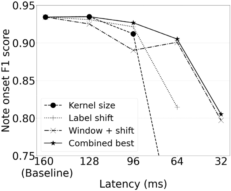
Fig. 5.

Note onset F1 score as a function of latency for various methods, categorized as models with reducing kernel size only (kernel size), models with label shifting (label shift), models with FFT window 1,024 and label shifting (window + shift), and the combination of the three methods that exhibited the best accuracy for a given latency (combined best). Only the best model of each method for given latency is presented. To enhance visual clarity, the Y-axis scale has been limited.

Reducing kernel sizes showed the best accuracy for the latency of 128 ms. Replacing size three kernel with size one kernel at the bottom layer of CNN stack showed the best F1 score, even slightly better than the baseline, albeit marginally. However, the accuracy drops to 91.20 % if the kernel sizes of two layers were reduced from three to one, which corresponds to the latency of 96 ms. The F1 score significantly drops to 63.52 % if we replace all the three kernels to size one.

Shifting labels showed better accuracy for latency of 96 ms and 64 ms compared to the reducing kernel sizes. However, the performance drop when shifting the label to the last frame of the receptive field (e.g., label shift 3 with the baseline model) was significantly large. We assume that one of the reasons is that the amount of audio sample after note onset can vary a lot if the model only uses a single frame of mel-spectrogram without using subsequent frames. For example, with the window size 2,048 and hop size 512, the amount of audio samples after note onset included in the onset-labeled spectrogram frame is between 768 to 1,280. If the onset occurs in the ending time boundary, the model has to detect the onset with only 40 % less audio samples compared to the onset that occurred in the beginning time boundary.

Reducing FFT window size from 2,048 to 1,024 showed lower accuracy for latency of 128 ms or 96 ms compared to kernel resizing or label shifting. We suppose the reason is because of degraded frequency resolution from lower FFT size. However, combining the reduced window size with label shifting and kernel reduction showed the best result for latency of 64 ms, note F1 score of 90.51 %, which is significantly higher than applying only kernel size modification (63.52 %) or label shift (81.45 %) with the same latency. The result shows that the window size has to be reduced to achieve a good performance with lower latency such as 64 ms.

Reducing hop size did not have a clear advantage over other methods. Also, considering that reducing hop size demands more computation power due to the increased frame rate, it would be carefully applied to the real-time application.

In summary, we found that each of the proposed methods has different optimal range where the accuracy preserved relatively stable. We observed that replacing one convolutional layer of kernel size three with kernel size one layer has relatively little impact on the accuracy. While the labeling shift approach is effective, it should be avoided if it results in label shifting to the last frame of the receptive field. In cases where the above methods have already reached their optimal limitation, reducing window size of FFT can be considered to further reduce the latency with optimal accuracy loss. Additionally, the large gap in accuracy among models with identical latency indicates that the transcription accuracy with low-latency is not solely determined by the number of required audio samples but also by the manner in which they are processed.

VI. Conclusion

In this paper, we experimented with several modifications to a previous neural network model for automatic piano transcription to reduce the latency in a real-time scenario. Three options were explored, reducing receptive field size, reducing window or hop size of FFT, and shifting the label during the training. Even though every option for reducing latency has a tradeoff with the transcription accuracy, we have found that mixing these options shows the best accuracy for a given target latency. For example, we could reduce the latency from 160 ms to 96 ms with losing note F1 score of less than 0.8 %p by reducing the kernel size of one convolutional layer and also applying label shift for one time frame. Also, combined with reduced window size, the modified model achieved note F1 score of 90.51 % with a latency of 64 ms. Even though the total system latency must account for additional variables such as computation time, reducing the intrinsic latency of the acoustic model can enable achieving a latency that falls within the acceptable range for applications such as ensemble performances.^[14]

Even though the experiment was based on a single architecture proposed by Kwon et al.,^[12] we expect that the proposed methodology can be applied to other transcription models. Also, the experiment result can help to design the proper kernel size or FFT parameters based on the use scenario of the AMT model. For example, if low latency is more important than high recall, one can use small window size and a shorter receptive field. The code is available in https://github.com/jdasam/low-latency-amt.