I. Introduction

Time delay estimation (TDE) between two (or more) received signals can be used as a means for the localization of the dominant source in applications such as receiver array beam steering for suppressing reverberation in all types of communication and voice processing systems.[1-3] There is a trend towards the use of multiple receivers in research and industry; however, the use of two receivers is present in actual applications such as humanoid robotics[2] and hearing aids.[4]

Most TDE methods rely on relative delays between the two receivers[5]. Although there are many effective TDE methods, the generalized cross-correlation (GCC) method, proposed by Knapp and Carter in 1976 [6], is the most popular technique for TDE. The delay estimate in this technique is obtained as the time lag maximizes the cross- correlation between filtered versions of the received signals. This method has been well studied and performs adequately[7]. Another interesting idea was proposed in [8] and it was further developed by Doclo and Moonen[9]. The algorithm in [8] estimates time delay using eigenvalue decomposition. The eigenvector that corresponds to the minimum eigenvalue of the covariance matrix of the received signals contains the impulse responses of the source and the received signals; subsequently all information necessary for time delay estimation can be derived from the eigenvector. However, it meets difficulty to select a single eigenvector for the minimum eigenvalue in the low SNR environments and correlated noise environments. This is because several small eigenvalues at roughly the same value are frequently found in the low SNR environments and correlated noise environments. In this case, the TDE performance degrades in the eigenvalue decomposition based algorithm in [8]. The algorithm in [9] improved the performance of the algorithm in [8] under the noisy environments by using an adaptive generalized eigenvalue decomposition (GEVD) algorithm. The usage of an adaptive GEVD in [9] needed to measure the pure noise signal. The GEVD introduced whitening effect to the algorithm in [8] so that it made it more better to derive a single eigenvector for the minimum eigenvalue.

Hotelling in [10] proposed a new multivariate analysis approach of Canonical Correlation Analysis (CCA). CCA was developed to measure the linear relationship of two multidimensional sets of variables. CCA has been widely used in economics, meteorology and in modern information processing fields, such as communication theory,[11] statistical signal processing[12] and blind source separation.[13] In [10] and [14], CCA can be defined as the problem of finding two vectors, w1 and w2, such that the variates y1= X1w1 and y2=X2w2 are maximally correlated with two multi-dimensional sets of variables of X1 and X2. Typically, CCA is formulated as a generalized eigenvalue (GEV) problem.

This paper proposes a more robust TDE algorithm than the eigenvalue decomposition based algorithm of [8]. In order to derive a new TDE algorithm using the eigenvector of the maximum eigenvalue rather than the eigenvector of the minimum eigenvalue, we can apply CCA concept to the proposed algorithm, because CCA can be defined as the problem of finding two vectors, w1 and w2, such that the variates y1=X1w1 and y2=X2w2 are maximally correlated with two multidimensional sets of variables of X1 and X2, as it is described above. In the proposed method, the CCA method is applied to the TDE by estimating vectors to maximize the linear relationship between the two received signal sets. We show that the eigenvector contains time delay information in 3.1, and formulate an adaptive algorithm to estimate the eigenvector for the maximum eigenvalue based on CCA. In order to derive an adaptive algorithm, we utilize the adaptive GEVD formulation in [9] as a solver. The proposed algorithm has no noise whitening effect although the noise whitening is a major contribution in [9]. In the simulation, we confirm the performance of the proposed TDE algorithm by comparing it with two different algorithms such as GCC and an adaptive eigenvalue decomposition based TDE. In the simulation, we consider normal independent white Gaussian noise case and correlated noise case. From the simulation, we confirm that the proposed algorithm works better than the eigenvalue decomposition based algorithm.

II. Models for the TDE Problem

This section discusses two models often used for the TDE problem. First, the ‘ideal model’ is described and then is followed by the ‘real model’ which more accurately describes a real acoustic environment.[8]

2.1 Ideal model

A simple and widely used signal model for the classical TDE problem is as follows. Let xi(k), i=1, 2, denote the i-th receiver signal, then: 

where αiis the attenuation factor due to propagation effects, τiis the propagation time from the unknown source s(k) to receiver i, and ni(k) is an additive noise signal at the ith receiver. It is assumed that s(k), n1(k), and n2(k) are zero-mean, uncorrelated, and stationary Gaussian random processes. The relative delay between the two received signals 1 and 2 is defined as.

2.2 Real model

In a real acoustic environment we must consider the reverberation of the room; therefore, the ideal model no longer holds. A more complicated but more complete model for received signals xi(k), i=1, 2, can be expressed as follows:

where * denotes convolution and gi is the channel impulse response between the source s(k) and the ith receiver. Moreover, n1(k) and n2(k) might be correlated which is the case when the noise is directional, e.g., from a ceiling fan or an overhead projector. This case is a very challenging problem that requires an accurate determination of the two impulse responses between the source and the two receivers.

III. The Proposed Method

3.1 TDE based on Canonical Correlation Analysis

In this work, transformation is performed on a sequence of features during speaking spurts.

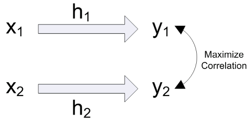
Let X1, X2 be two known full-rank data matrices of size M×N and M×N, respectively. In Fig. 1, CCA can be defined as an approach to solve the problem of finding two vectors: h1 of size N×1 and h2 of size N×1, such that the variates and are maximally correlated, i.e. [13],

where is an estimate of the correlation matrix.

The aforementioned CCA concept can be utilized to the time delay estimation between two different receiving sensors. Assuming x1 and x2 are the received signal vectors in the receiving sensors in the size of N×1, h2 means the mapping channel between x2 and y2, and h1 means the channel between x1 and y1. The mapping channel h1 and h2 maximize the correlation between y1 and y2 with delays, D1 and D2. The mapping channels operate as follows.

When the correlation between y1(k) and y2(k) becomes maximum, the relationship between the delays in the received signals and the delays in the mapping channels satisfies as follows.

Therefore, the difference between the peaks of h1 and h2,becomes the relative time delay between x1 and x2 as (2).

Problem (4) can be formulated as the following constrained optimization problem.[13]

The solution of (8) is given by the eigenvector corres-ponding to the largest eigenvalue of the following generalized eigenvalue problem.[14-15]

where ρ is the maximum correlation between the two sets of variables and  is the eigenvector. Adding to both sides in (9), we can modify (9) as follows:

In (11), the eigenvalue will be obtained as ,[16] where is the maximum correlation coefficient. Even though x1 and x2 are noisy, the additive noise effect to the correlation coefficient is negligible because the additive noise is mutually uncorrelated white noise. The maximum eigenvalue is less affected by the additive noise; therefore, the estimated eigenvector of the maximum eigenvalue is more robust against the additive noise in the proposed algorithm. This makes the proposed algorithm superior to the adaptive eigenvalue decomposition based method that uses the eigenvector of the minimum eigenvalue.

The mapping channels, h1 and h2, are derived from the eigenvector, v, corresponding the largest eigenvalue. Alternatively, the eigenvector corresponding to the largest eigenvalue in (10) can be obtained as the eigenvector corresponding to the smallest eigenvalue of the following equation;

Adding to both sides in (13), we can modify (13) as follows:

(14) can be developed to much easier adaptive formulation. We will show it in the following subsection.

3.2 Adaptive GEVD algorithm for CCA based TDE

For the solution procedures on the GEVD, in (14), it is also possible to derive stochastic gradient algorithms that iteratively estimate the generalized eigenvector that corresponds to the smallest generalized eigenvalue of B and A.

Instead of updating the full GEVD of B and A [17] and then deriving generalized eigenvector that corresponds to the smallest generalized eigenvalue, it is possible to iteratively estimate this generalized eigenvector by minimizing the cost function vTBv subject to the constraint vTAv = 1, where and . This problem can be solved by minimizing the mean square value of the error signal e(k),

where .

The iterative procedure can be done using a gradient-descent LMS procedure in [9] and [18],

with μ the step size of the adaptive algorithm. The gradient of e(k) now is equal to (17).

Substituting (17) and the constraint, vTAv = 1, into (16) gives (18).

where In order to avoid round-off error propagation, we normalize the updated vector, , as (19).

For better convergence, we can utilize the normalized LMS approach with (18) as (20) [18].

In each iteration, we can derive the estimation value of the time delay from the difference between two peak value positions in and in . The expected TDE can be computed as the difference between the two peak value positions in and . We also try to improve the numerical stability by adding a small value to the diagonal of matrix. Table 1 summarizes the proposed algorithm.

IV. Simulation and Comparison

We began with generating two signals. In most practical applications, the desired source signals of interest are correlated. The source signal x1(k) was generated by passing a first order AR process, viz., s0(k) = 0.7s0(k) +w(k), where w(k) is a white Gaussian process.[19] Assuming the signals propagated in the free space, the second signal x2(k) is the time-delayed version of x1(k)= s0(k) with delay D=10, i.e. x2(k)=x1(k−10). Then, the two signals x1(k) and x2(k) are contaminated by two real white Gaussian noises n1(k) and n2(k), respectively. We check to ensure that the two noise sequences are mutually uncorrelated. In this simulation, we set the channel dimension of h1 and h2 to 100 and the data matrix X1, X2 is reduced to data vector x1, x2 of 100×1, respectively, because the proposed algorithm estimates the channel h1 and h2 recursively instead of batch processing.

The signal sequences were scaled to obtain the desired SNR and added to the noise sequences as in (1) to form the sensor outputs x1(k) and x2(k). SNRs of approximately from 20 dB to -10 dB were considered, where SNR=.

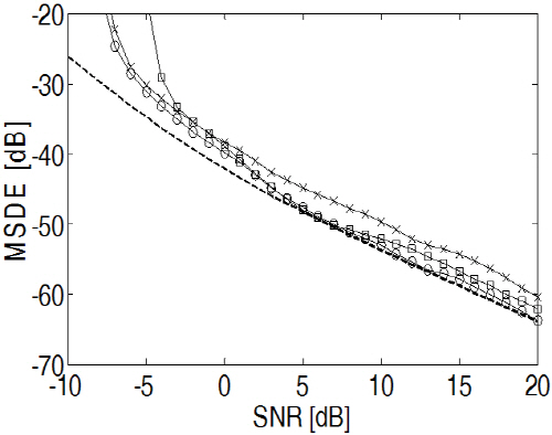
The sequences x1(k) and x2(k) were processed using the traditional GCC,[6] adaptive eigenvalue decomposition based method[8] and the proposed method. We compared the mean squared delay errors (MSDE) for the performance comparison. All the results provided were averages of 1000 independent trials. Fig. 2 shows the MSDE of the three algorithms and compares them with Cramér-Rao lower bound (CRLB).[13] When SNR≥0 dB, the proposed method and the adaptive eigenvalue decomposition method are better than the GCC. When SNR< -3 dB, the performance of the adaptive eigenvalue decomposition method suddenly deteriorates; however, the proposed method still provides good performance. When SNR drops down to -10 dB, all of the TDE algorithms begin to deteriorate. Especially, as an eigenvector based method, the proposed method is more robust against noise than the adaptive eigenvalue decomposition based method. The better performance is because the proposed algorithm estimates the time delay by the eigenvector of the maximum eigenvalue.

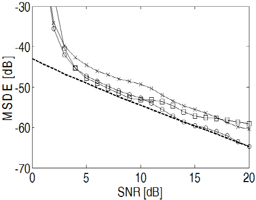
In the second experiment, the case of the correlate noises was considered. This case frequently happens when the noise is directional such as from a ceiling fan or an overhead projector. We generated correlated noise as i.e. n1(k)=n2(k-5), where n2(k) is real white Gaussian noise. We also compared the MSDE for the performance comparison by 1000 independent trials. SNRs from 20 dB to 0 dB were considered, because all the algorithms failed below 0 dB. Fig. 3 shows the MSDE of the three algorithms: When SNR≥ 3 dB, the proposed estimator outperforms the GCC. When SNR≤10 dB, the proposed estimator is parallel with the adaptive eigenvalue decomposition method. When SNR>10 dB, the proposed method performs superior to the adaptive eigenvalue decomposition based method. From these results, we can conclude that the proposed method is a good time delay estimator.

V. Conclusion

This paper proposed a new approach to time delay estimation. The method derives the time delay parameter from the eigenvector for the maximum eigenvalue estimated by canonical correlation analysis of the receiver signals. In comparison with other methods, the proposed algorithm is more robust in reverberation environments as well as in uncorrelated noise environments and correlated noise environments.

In further research, we will study the performance comparison between the proposed algorithm and the algorithm in [9]. We think that it is worthwhile to compare the two algorithms in the following aspects:

-Two algorithms use an adaptive GEVD formulation.

-The proposed algorithm uses an eigenvector for a maximum eigenvalue.

-The algorithm in [9] uses an eigenvector for a minimum eigenvalue.

-The proposed algorithm needs no noise whitening.

-The algorithm in [9] needs noise whitening so that it should measure the pure noise signal.