

I. Introduction
II. Modified FxLMS algorithm
2.1 Sun’s algorithm
2.2 Akhtar’s algorithm
III. Intelligent ANC SYSTEM
3.1 Probability estimation
3.2 Zero-crossing rate control
3.3 Optimal parameter selection based on fuzzy control
IV. Computer Simulation
4.1 Case 1
4.2 Case 2
V. Conclusions
I. Introduction
Acoustic noise problems become more and more evident. But the passive techniques in acoustic noise control such as enclosures, barriers, are relatively large, costly, and ineffective at low frequencies. ANC based on cancellation of acoustic waves [1] can efficiently attenuate low frequency noise with benefits in size and cost.
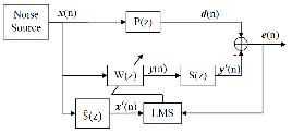
The famous FxLMS algorithm[2] is shown in Fig. 1. Essentially, ANC system cancels the primary noise by generating and combining an anti-noise (with equal amplitude but opposite phase).[1,3] For generating this anti-noise, we use adaptive filter  to estimate the unknown primary transfer function
  by minimizing the mean square error
  ; the reference signal
  is received by microphone; and then, we generate digital anti-noise signal
  ; this digital signal is transformed to a real anti-noise
  in an acoustic domain after passing through the secondary path
  . The update equation of adaptive filter
  is
is
 ,
,where  is the step size,
  is the filtered
  signal by
  , but
, but  is unknown and must be estimated by an additional filter
  .[2]
.[2]
The FxLMS algorithm may become unstable, especially in a non-stationary impulsive noise environment.[4] To solve this problem, Sun proved that the samples of the reference signal should be treated probabilistically.[4]
Sun’s algorithm and Akhtar’s algorithm[5] used the assumption that the noise has a uniform distribution within a certain range, then they ignored (or clipped) the noise out of this range. In their experiments, they selected the threshold parameters offline and improved the stability for a special impulsive noise environment. But these two algorithms have dissatisfied performance and stability in huge magnitude or sustaining impulsive noise environment.
To improve the performance, we propose an estimated probability density function (PDF) of reference signal; to improve the stability, we control the adaptive filter’s step size according zero-crossing rate; and to select optimal threshold in various noise environments, we develop an online parameter selection method based on fuzzy system.
The organization of this paper is as follows. Sun’s algorithm and Akhtar’s algorithm are briefly described in Section II. Section III introduces the proposed algorithm. In Section IV, the simulation results are illustrated comparing with the existing algorithms. Conclusions are drawn in section V.
II. Modified FxLMS algorithm
FxLMS algorithm may become unstable in non-stationary impulsive noise environment. Some algorithms have been researched to solve this problem. One is based on minimizing least mean pth-power (FxLMP) of the error signal[6]; the others are based on modifying the reference signal during the update of FxLMS algorithm. Sun’s algorithm and Akhtar’s algorithm are the later approach.
2.1 Sun’s algorithm
Sun proved that the samples of the reference signal  should be treated probabilistically as follow
 ,
,where  denotes linear convolution,
  is the PDF of reference signal. This PDF can not be calculated, so the assumed one in Fig. 2 is used. The thresholds
  and
and  are obtained in offline operation. Thus
  is modified as
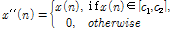 .
.After this modification, Sun’s algorithm is given as
 .
.2.2 Akhtar’s algorithm
Akhtar’s algorithm[2] is a modified and extended version of Sun’s algorithm, the reference signal is modified as
 .
.He also extended this idea to error signal  as shown
 .
.Akhtar’s algorithm is given below
 .
.III. Intelligent ANC SYSTEM
Although Sun’s algorithm and Akhtar’s algorithm increase the robustness, the stability and performance are still not satisfied, especially, when they deal with sustaining impulsive noise. To solve this problem, we develop probability estimation and zero-crossing rate control; and to eliminate the effect of impulsive noise, an optimal parameter selection based on fuzzy control is also utilized.
3.1 Probability estimation
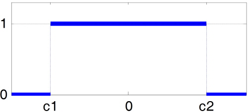
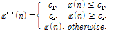
In Sun’s and Akhtar’s algorithms, they assumed the noise has a uniform distribution within the range  and then ignored the noise out of this range. However, the proposed algorithm is different, we use the range
  instead of
  . Then we assume that the probability of the noise beyond this range exists but decreases rapidly,[7] as
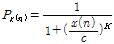 ,
,where  is the attenuation factor and controls the attenuation speed. In proposed algorithm, we experimentally choose
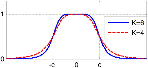
  equals 6. The estimated PDF of
  is shown in Fig. 3. To compare the attenuation speed, the PDF of
  is also shown in this figure.
Actually, in proposed algorithm, we utilize a forgetting factor  (0.9 <
 < 1) to smooth the probability of adjacent samples.
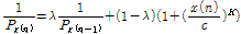 .
.Using this probability estimation, the update equation of FxLMS algorithm is modified as
 .
.3.2 Zero-crossing rate control
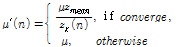
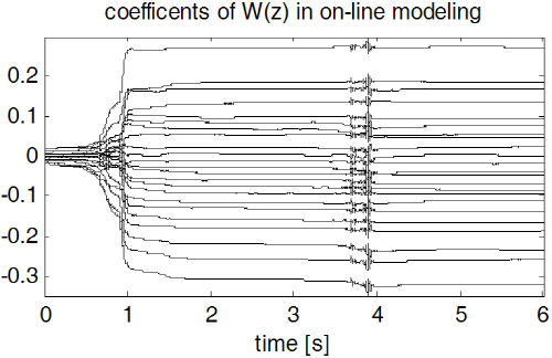
During experimental implementation, we observe that the coefficients of adaptive filter are sensitive and change rapidly when the ZCR of current signal is relatively high as around 0.9 s and 3.8 s in Fig. 4.
This phenomenon has dual characters. It may help adaptive filter converge quickly at about 0.9 s; or it may lead to a crash after the algorithm has converged at approximately 3.8 s.
According to this phenomenon, zero-crossing rate control is employed after the algorithm has converged.
 .
.where  is the zero-crossing rate around current sample and
  is the mean zero-crossing rate of the noise.
The update equation of FxLMS algorithm is modified to
 .
.3.3 Optimal parameter selection based on fuzzy control
The threshold parameter  in (8) controls the estimated probability of the reference signal. A small
  will treat normal noise as low probability signal, likewise, a large
  can not reduce the mischief of impulsive noise, so the choice of
  have much more effect on the performance. Our idea is that when impulsive noise appears we shrink
  to reduce the effects of this impulsive noise. We propose fuzzy control to utilize this idea. The simulation results in next section show that we successfully eliminate the effects of impulsive noise with a relatively small threshold and preserve the information of normal noise with a relatively large threshold.
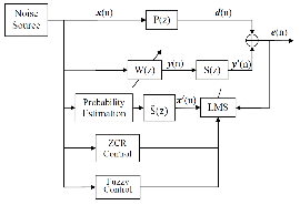
Our fuzzy logic controller has two inputs and one output. For fuzzification, the isosceles triangle and max-min method are used.[8] For defuzzification, the center of area method is used.
The first fuzzy input variable  is defined as the ratio between current signal magnitude
  and mean magnitude value
  of stationary noise.
 .
.Second fuzzy input variable  is defined as the duration (in samples) of current signal magnitude.
The output of fuzzy controller is  , it is the coefficient of
  . The threshold
  can be calculated as follow
 .
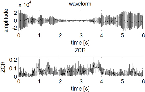
.The linguistic variable in  ,
,  and
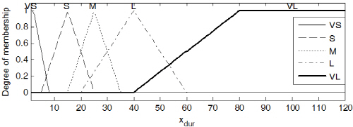
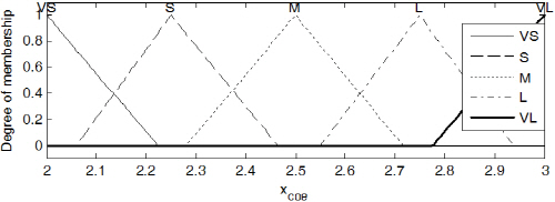
and  are shown in Table 1 and the membership functions are shown in Fig. 5.
 and
and  .
.
 and
and  .
.Fuzzy approximation uses IF ~ Then rule. Our rules are decided based on experiments and shown in Table 2. The block diagram of proposed algorithm is shown as follow
IV. Computer Simulation
This section provides the simulation results to verify the effectiveness of the proposed algorithm comparing with Sun’s algorithm and Akhtar’s algorithm.
 \
\
All reference signals we used are actual noise. In our simulations, the primary path  and the secondary path
  in Fig. 1 are IIR filter and the filter parameters can be found in the disk attached to with Ref.[2]. The length of adaptive filter we selected is 256. We use noise ratio(NR) as performance measure.
  is defined as
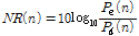 ,
,where  and
and  are the powers of residual error signal
  and disturbance signal
  .
.
4.1 Case 1
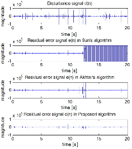
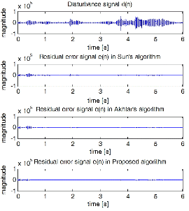
The reference noises for Case 1 are car noises. We pick out 19 car noise signals with lots of instantaneous and sustaining impulses. The average length of these noise signals is 20 seconds. After implementation with these signals, Sun’s algorithm is unstable for 10 realizations, Akhtar’s algorithm is unstable for 6 realizations, as compared with them, the proposed algorithm is stable for all realizations.
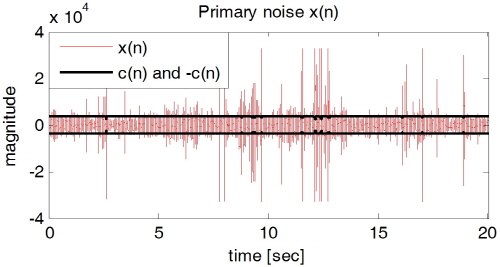
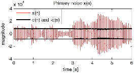
One of the noise signal is shown in Fig. 7. The results given in Figs. 8 and 9 demonstrate that the proposed algorithm gives the best performance, stability and convergence speed.
4.2 Case 2
In this case, factory noises are recorded as reference noises. We pick out 20 noise signals, one of them is shown in Fig. 10. These factory noises have few impulses, but the noise magnitude is changing quickly. Dealing with this kind of noise, Sun’s algorithm and Akhtar’s algorithm are stable, but their convergence speed are quite slow.
The average length of these noise signals is only 6 seconds, but the sampling frequency is higher than in Case 1. The results of noise signal in Fig. 10 are shown in Fig. 11 and Fig. 12.
From Case 1 and Case 2, Sun’s algorithm and Akhtar’s algorithm are relatively unstable and have dissatisfactory stability in dealing with sustaining impulsive noise, the proposed algorithm has much more better performance, stability and convergence speed in non-stationary noise environment.

 ), Akhtar’s algorithm (
 ), and proposed algorithm(
 ) respectively.
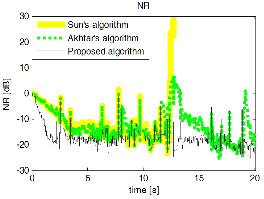
 ), Akhtar’s algorithm(
 ), and proposed algorithm(
 ) respectively.
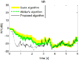
V. Conclusions
The proposed algorithm is based on modification of FxLMS algorithm. We proposed probability estimation and zero-crossing rate control to improve the stability and performance. In Sun’s and Akhtar’s algorithm, they used a special noise environment and estimate the threshold parameters offline. To ameliorate it, we developed an online parameter selection method based on fuzzy control. Comparative simulation results demonstrated the proposed algorithm has improved the stability, performance and convergence speed.
