I. Introduction
II. Data Overview and Description
III. Whistle sound extraction and time frequency contour classification
IV. Contour shape classification
V. Whistle comparison result
VI. Conclusion and further discussion
Appendix
I. Introduction
The false killer whale (Pseudorca crassidens) is distributed throughout tropical and sub‑tropical seas worldwide, feeding primarily on fish and squid.[1,2,3] False killer whale is classified as ‘Endangered’ by the International Union for Conservation of Nature (IUCN), highlighting the conservation importance of this species.[4] Around the Hawaiian Archipelago, three major populations of false killer whales are known to exist: those inhabiting the Main Hawaiian Islands (MHI), the Northwestern Hawaiian Islands (NWHI), and the pelagic region.[5]
Among these, the MHI stock was the first to be recognized and comprises false killer whales that reside around the main Hawaiian Islands.[6,7,8,9,10,11,12,13,14] The NWHI stock was identified in 2013,[11] and subsequent genetic analyses confirmed that gene flow between stocks is minimal.[12] In addition to these island-associated stocks, a widely distributed pelagic population occupies offshore waters of the archipelago and overlaps spatially with both the MHI and NWHI stocks, providing an important broader-ocean context for interpreting island-associated differences.[12] Such genetic and ecological divergence raises the possibility of corresponding acoustic differences among populations, and analyzing these differences can be an important tool for understanding their degree of separation.[5]
False killer whales generally produce three main types of acoustic signals—clicks, burst pulses, and whistles—that support communication and foraging.[14,15,16] Whistles, in particular, are informative for examining social bonding and survival strategies because their frequency range, duration, and time‑frequency variations can reflect social and ecological adaptations.[14,15,16]
A previous study attempted to classify the three Hawaiian populations using whistle measurements.[14] The average correct classification rate across all three populations was 42 %, with the highest average rate for MHI whistles (52 %) and the lowest for NWHI whistles (36 %); pelagic whistles averaged 42 %.[14] Pairwise classification improved modestly for pelagic vs. MHI (62 % average accuracy).[14] The results of this study suggest that the endangered MHI population may exhibit differences in the acoustic characteristics of its whistle compared to other populations. Analyzing these differences can contribute to understanding the differentiation and ecological differences between the three populations and to species conservation.[14]
This study aims to examine whether whistle characteristics differ among three populations of false killer whales inhabiting around the Hawaii, and to release whistle analysis data to support future research. To achieve this, we utilized “9th International Workshop on Detection, Classification, Localization, and Density Estimation (DCLDE) 2022” data set, which is well suited for broad scale regional comparison. The most accurate way to extract the characteristic signal feature of whistles (i.e., time-frequency contours) is through manual extraction.[17,18,19] In this study, we manually extracted the time–frequency contours, as manual annotation currently provides the most accuracy for contour identification. All extracted whistles were visually inspected and classified into six categories based on their time-frequency shapes. We compared whistle properties (e.g., duration, minimum/maximum/start/end frequency, and bandwidth) across time–frequency shapes and among the three populations. To handle unbalanced sample sizes and unequal variances typical of field recordings, we utilize Welch’s Analysis of Variance (ANOVA) tests and bootstrap, and we summarized effect sizes using Cohen’s d to interpret biological relevance.
The main contributions of this paper can be summarized as three points. First,manual extraction of whistle time–frequency contours based on MHI, NWHI, and pelagic populations. Second, analysis and verification of mean differences in whistle characteristics according to time-frequency shapes of three populations. Third, public release of the extracted False Killer Whale whistle contour dataset to facilitate reproducibility and future research.
This paper is organized into six sections. Section II describes the dataset used in this study, and Section III outlines the whistle contour extraction and Section IV describes time-frequency shape classification methods. Section V describes comparison results of the whistle characteristics based on time-frequency contour, and Section VI concludes the paper.
II. Data Overview and Description
In this study, we used recordings of false killer whales provided by the 9th International Workshop on DCLDE 2022 workshop.[20] The dataset was collected in 2017 around the Hawaiian Islands as part of Hawaiian Islands Cetacean and Ecosystem Assessment (HICEAS).[20] A towed acoustic system was employed for data acquisition, which consisted of a towed hydrophone array, an SA Instrumentation Data Acquisition (DAQ) sound card, a laptop computer, and PAMGuard software.[20] The towed array comprised two sub-arrays, each housing three hydrophones with an average sensitivity of –144 dB (@2 ~ 100 kHz). The signals were digitized with 16-bit quantization at a 500 kHz sampling rate. Data collection occurred over four months, from July to November 2017, and was supported by expert visual observations and acoustic analyses that ensured high reliability.[20] However, individual animal identities are not available in the HICEAS 2017 dataset. We analyse the pooled set of whistles recorded from each population over multiple encounters, months and sites as a comprehensive sample that summarizes the overall distribution of basic whistle characteristics for that population. Therefore, the resulting statistics from these data are better suited to describing broad regional differences in whistle characteristics across observed sample designs, rather than drawing detailed inferences at the individual animal or group level. For more accurate analysis, we excluded recordings collected from areas where population ranges overlap and recordings in which other cetacean species were detected concurrently.
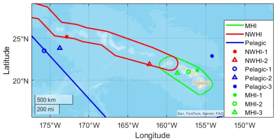
Fig. 1 shows the recording locations of false killer whale whistles in the DCLDE2022 data set together with the activity ranges of the three populations (MHI, NWHI, and pelagic). In Fig. 1, green, red, and blue indicate the activity ranges of the MHI, NWHI, and pelagic populations, respectively.[21]
The time windows used for whistle time-frequency contour extraction at each site are summarized in Table 1.
Table 1.
Site information and contour extraction ranges.
Consequently, whistle time-frequency contours were extracted from two sites for NWHI and from three sites each for the pelagic and MHI populations.
III. Whistle sound extraction and time frequency contour classification
To analyze false killer whale whistle sounds, it is necessary to extract their time-frequency characteristics. However, these recordings often include over-lapping whistles and clicks in the time-frequency domain, along with ambient noise. These factors make it challenging to isolate whistle contours. For this reason, conventional studies adopted manually extracted whistle contours as the reference standard, showing that they surpass automated approaches in accuracy.[17,18,19] Thus, manually extracted whistle contours were used as training data.[18] Accordingly, in the present study, we manually extracted the time-frequency contours of false killer whale whistles from the DCLDE 2022 dataset. We extracted the whistle contours from the spectrogram. To generate the spectrogram, we used MATrix LABoratory (MATLAB) and down sampled the recorded signal from 500 kHz to 50 kHz. We used a 4096-point Fast Fourier Transform (FFT) with a Hamming window, shifting the window every 2 s.
Manual contour extraction protocol. Five researchers extracted whistle contours following this protocol. Contours were extracted only when the same time–frequency shape could be visually confirmed on at least three hydrophones. Among the six arrays, the array exhibiting the highest Signal to Noise Ratio (SNR) was identified from the spectrogram, and the contour was extracted from that array’s spectrogram. To assess consistency, whistle contours were independently extracted by all researchers involved in the extraction from the same 5-minute raw data segment, and more than 70 % agreement was observed across them. The MATLAB code used for manual extraction has been made publicly available.
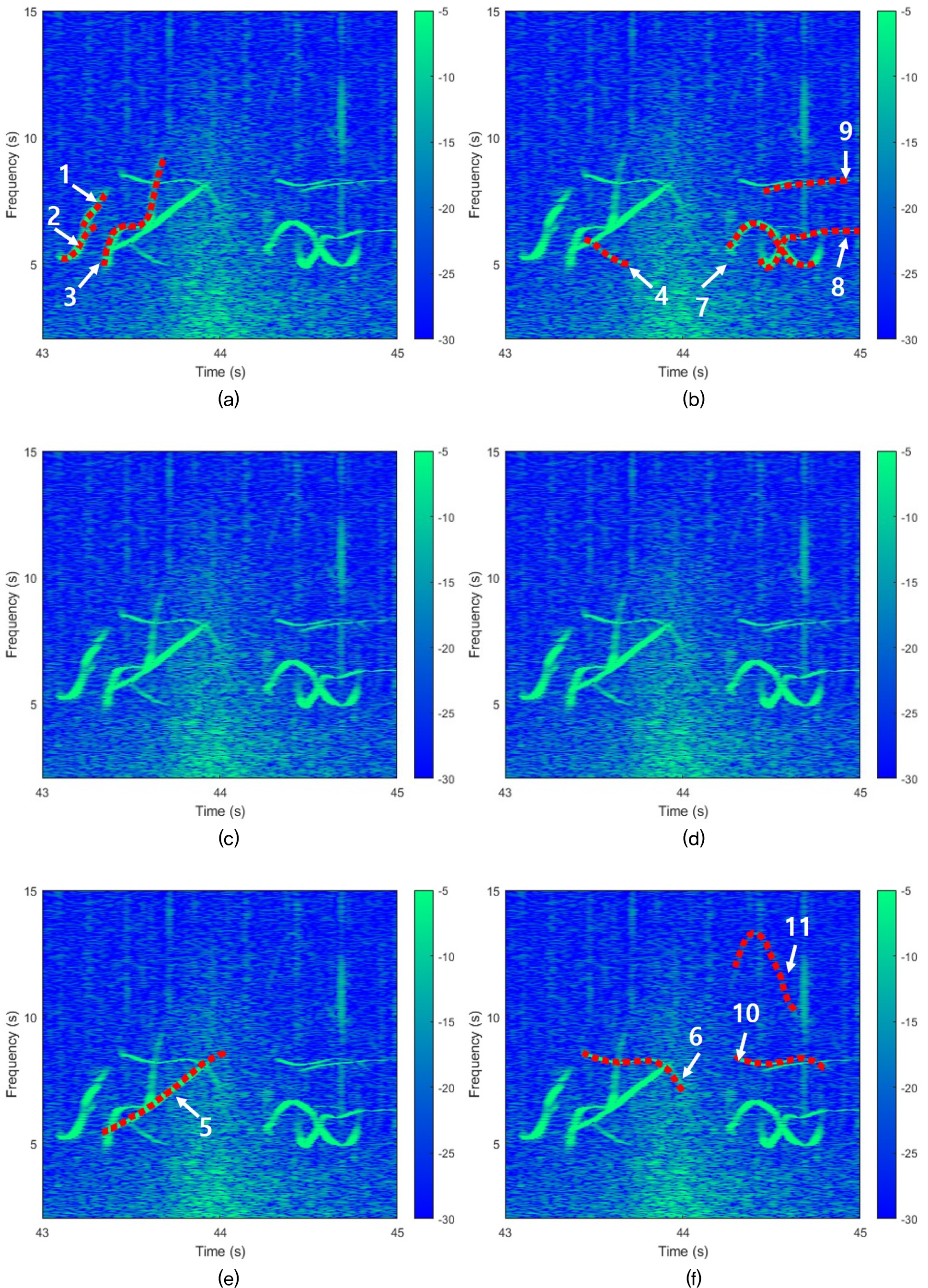
Fig. 2 presents an example of a manually extracted false killer whale whistle contour recorded data from Pelagic-2 between 00:06:35 and 00:07:35 recoding file in Table 1. Red dot lines indicate the manually extracted whistle contours. A total of eleven whistles are visible in the spectrogram. For the first, second and third whistles, the lowest background noise was observed in the spectrogram from array 1, so their contours were extracted from that array. The eleventh whistle has a low SNR and is faintly visible to the naked eye. However, because the same whistle pattern was simultaneously observed across three or more arrays, its presence can be reliably confirmed. Even if the whistle has a low SNR, if the same shape is observed in three or more of the six arrays, it is judged to exist and extracted.
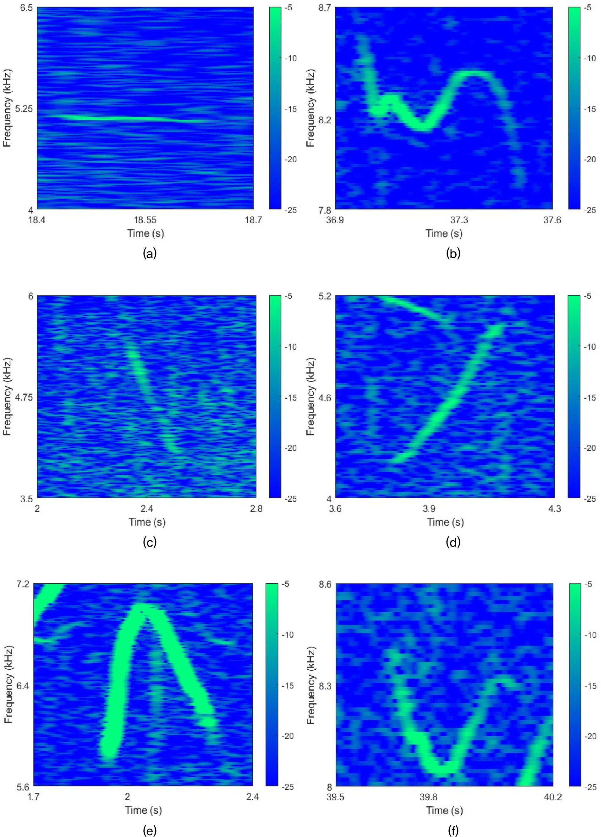
Using this approach, we manually extracted false killer whale whistles from recordings at eight locations. According to previous study, false killer whale whistles can be categorized into six types.[2] Fig. 3 shows representative shapes of these six whistle contour shapes. These examples are spectrograms also recorded from Pelagic-2.
The contour shape classification procedure is presented in detail in Section IV.
IV. Contour shape classification
False killer whale whistles were ultimately assigned to six contour shapes through a three steps hierarchical iterative procedure: (1) selecting clear prototype whistles for each contour shape, (2) assigning whistles with unambiguous visual shapes using these prototypes and their feature vectors, and (3) iteratively re‑examining the remaining ambiguous whistles using additional features until they could be assigned to one of the six shapes.
First, whistles with clearly defined shapes in the spectrogram were selected to establish initial prototypes for each contour shape, and a feature vector (e.g., comprising duration, extreme frequencies, initial and terminal slopes, curvature index, and related metrics) was extracted from these prototypes. Fig. 4 shows the distribution of feature values extracted from whistles whose shapes were clearly distinguishable by human annotators at the time of extraction.
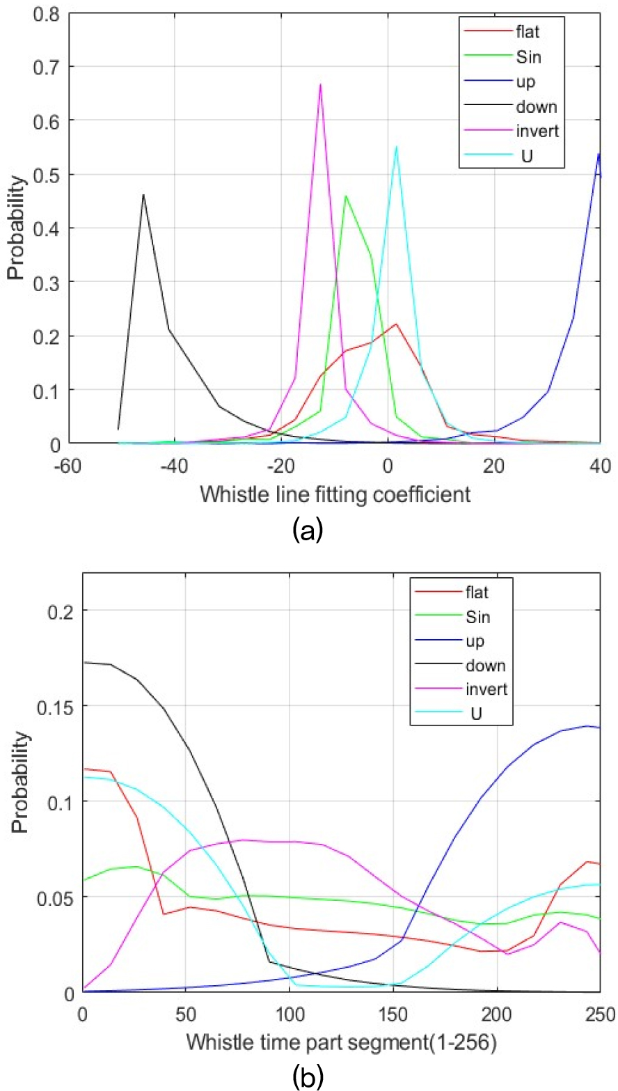
Fig. 4(a) shows the distribution of slope values, where each slope was obtained by approximating an individual whistle contour with a first-order linear fit. In other words, we fitted a straight line to each contour, extracted its slope, and then organized these slope values according to the contour shape categories. Fig. 4(b) presents the distribution of the maximum frequency position after each whistle contour was divided into 256 equal time bins. As shown in Fig. 4(a), up and down whistles are clearly separated by the line fitting coefficient, whereas this variable does not distinguish other contour shapes. Therefore, an additional discriminative feature is required. The position of the maximum frequency in Fig. 4(b) fulfills this role. Inverted U whistles generally reach their highest frequency near the midpoint of the contour, whereas U shaped whistles peak near either end. This characteristic enables us to separate the two shapes. Whistles that still lacked a clear label were gathered and re-examined until a suitable feature was found. Through these iterations, all whistles were ultimately assigned to one of the six contour shapes. Because the classification code and results have been publicly released, further details can be found by referring to the distributed code. The classification results are provided in Table 2.
Table 2.
Number of extracted whistles time-frequency contour based on time-frequency shape.
| Shape | NWHI | Pelagic | MHI |
| Flat | 1615 | 8346 | 349 |
| Sin | 300 | 2754 | 170 |
| Down sweep | 1372 | 5668 | 665 |
| Up sweep | 1922 | 11470 | 572 |
| Invert U | 2227 | 8394 | 593 |
| U shape | 917 | 8196 | 431 |
| Total | 8353 | 44828 | 2780 |
Using this fully classified set, we analysed the occurrence frequency of each contour shape among the three populations. The results are shown in Fig. 5.
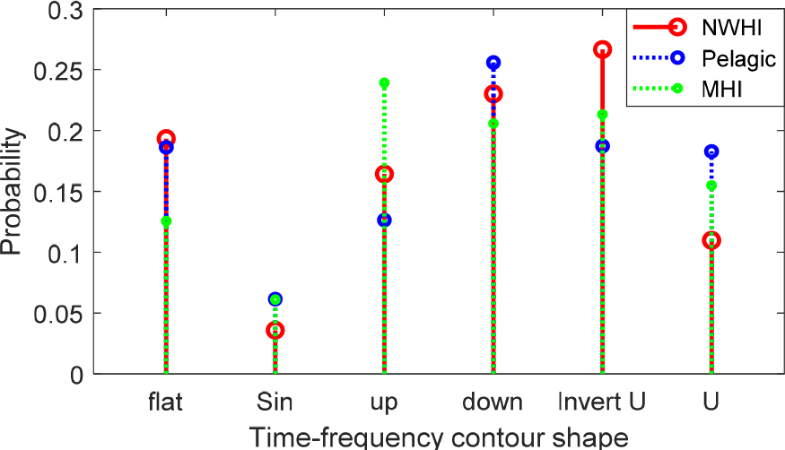
There were differences between the MHI and the other two populations in flat and up. The occurrence of up-shaped whistles was higher in the MHI than in the two other populations, but the occurrence of flat whistles was lower in the MHI than in the other two populations. The occurrence of down and sinusoidal whistles was similar among the three populations. In particular, the sinusoidal whistle was the least frequent in all three populations.
The frequency of U and inverted U-shaped whistles was different in the NWHI population than in the other two populations. The occurrence of inverted U-shaped whistles was higher in the NWHI than in the two other populations, but the occurrence of U-shaped whistles was lower in the NWHI than in the other two populations.
V. Whistle comparison result
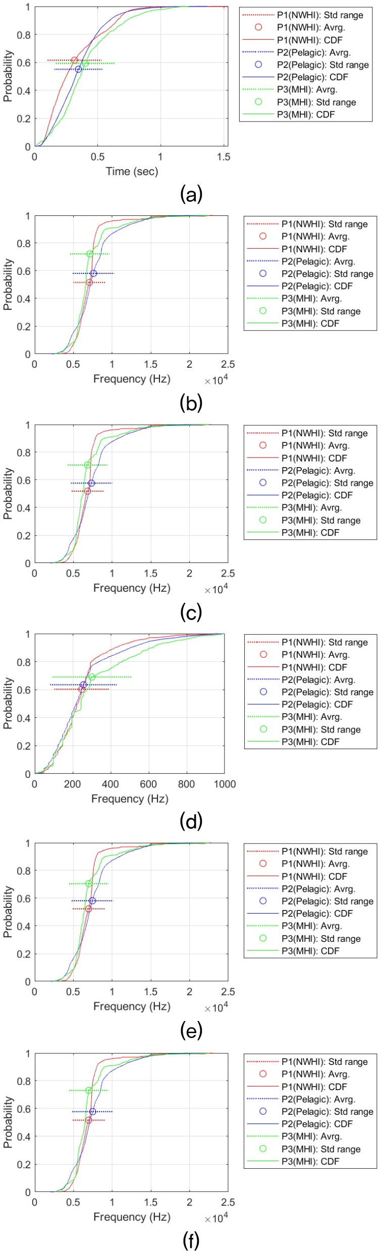
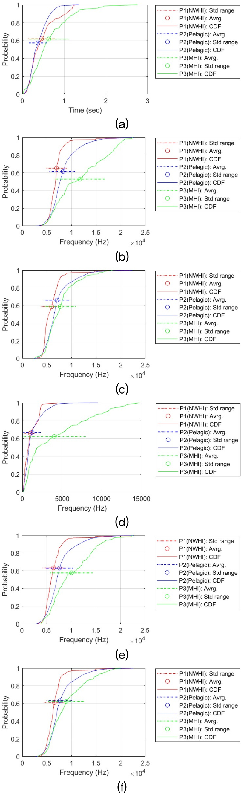
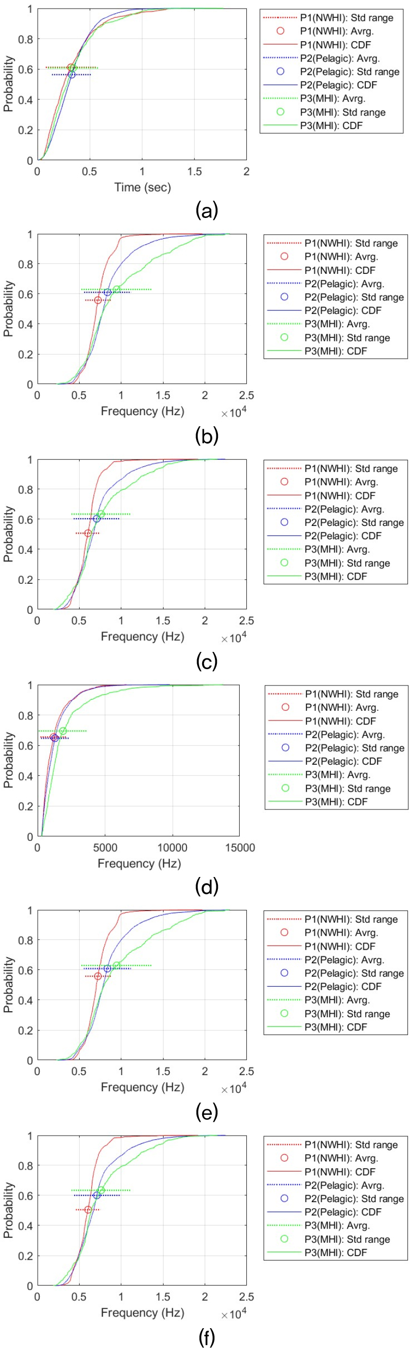
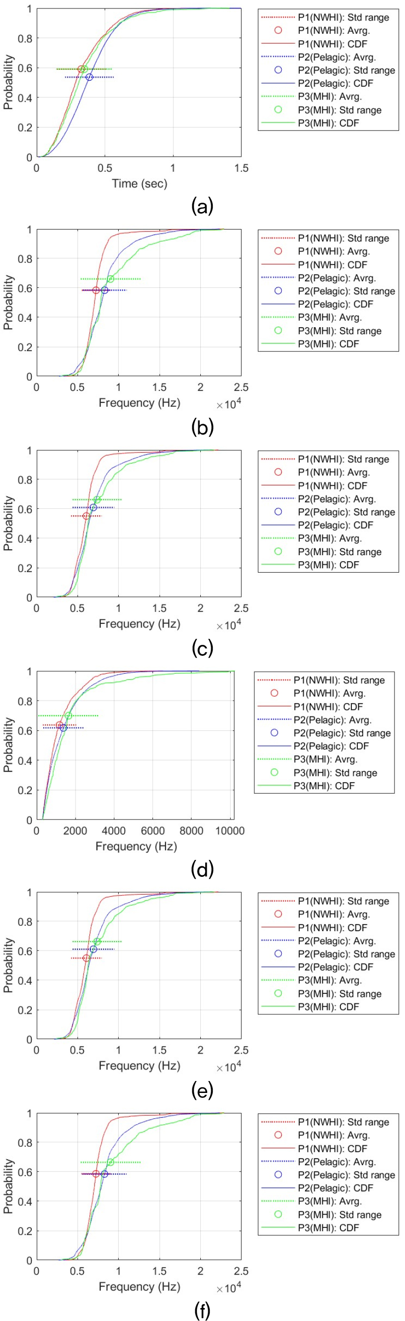
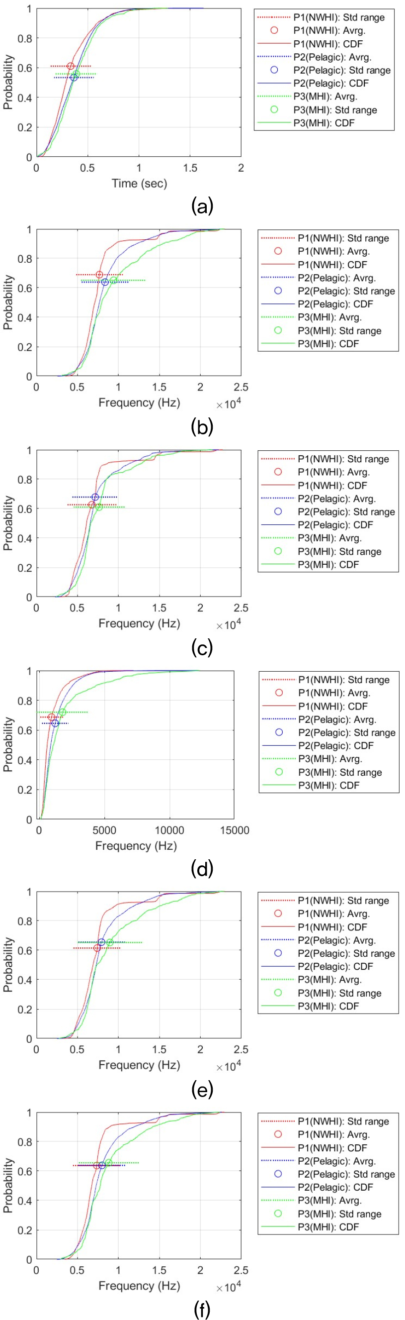
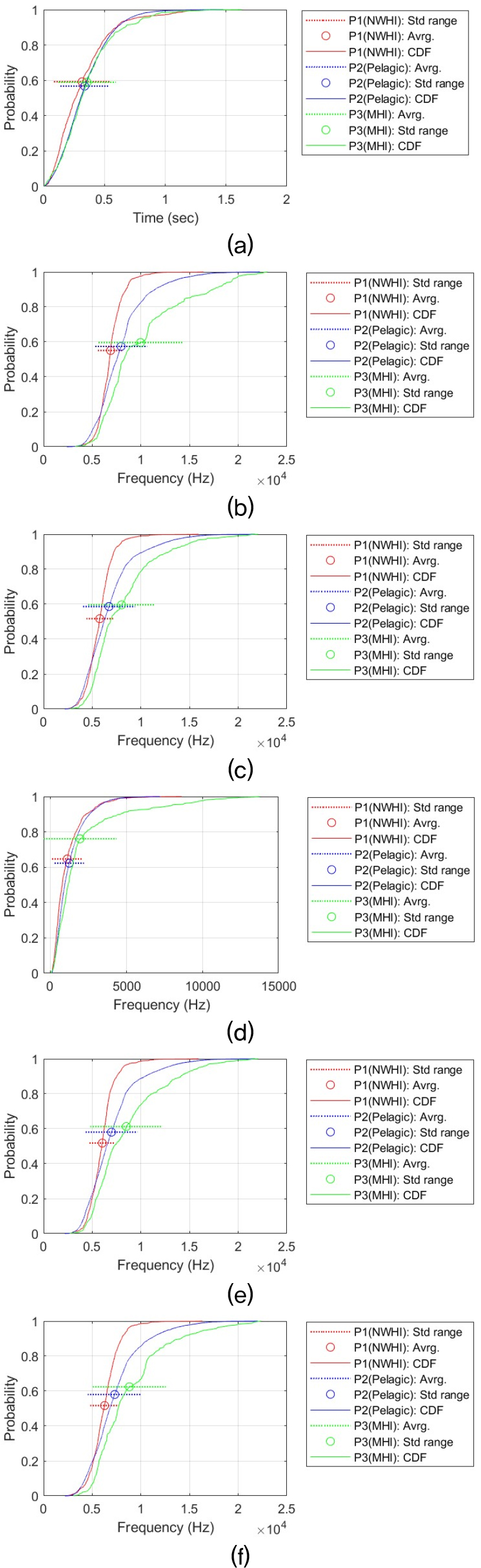
Acoustic features are selected to investigate the statistical properties of false killer whale whistles. These features are the time duration (Dur), maximum frequency (MaxF), minimum frequency (MinF), frequency bandwidth (BanF), start frequency (StaF), and end frequency (EndF). By comparing these whistle features, we determine whether there are actual differences among the three populations. We first measured the Cumulative Distribution Functions (CDFs) of each whistle feature by contour shape. We additionally performed statistical tests to assess whether the observed differences among populations were statistically significant, and we calculated effect sizes to evaluate how large those differences were.
The statistical tests performed in this paper were designed to compare means across populations. To achieve this, we first checked whether the three populations had equal variances for each characteristic. We confirmed unequal variances in all signal characteristics across the three populations using the Brown–Forsythe test, and then performed Welch’s ANOVA.
This statistical analysis process was performed for each time–frequency contour shape and each of the six signal features (Dur, MaxF, MinF, BanF, StaF and EndF), resulting in 36 separate Welch’s ANOVA tests. If 36 independent tests are all conducted at a nominal significance level of 0.05, the family‑wise error rate would inflate to approximately 84 %, meaning that at least one false positive would be expected by chance alone under the global null. To control this, we applied the Holm–Bonferroni procedure across the set of 36 ANOVA p‑values when assessing statistical significance.[22]
After ANOVA, Post‑hoc pairwise comparisons were performed with the Games–Howell procedure, which controls the family‑wise error rate under unequal variances and unequal number of samples.[23] For each pair we report the mean difference (Δ) and Cohen’s d, together with 95 % bootstrap CIs obtained via stratified within‑group resampling with 1,000 times. Bootstrap to handle imbalance.[24] For each comparison, we drew equal‑size samples per region (size = min available across the three), with 1,000 bootstrap iterations. We report the bootstrap 95 % CIs for mean differences and Cohen’s d. This reduces leverage from the larger Pelagic sample and keeps the comparisons conservative and reproducible.
Consequently, the magnitude of the differences in whistle signal characteristics across each population can be interpreted, along with confidence intervals. In summary, this analysis (i) verifies whether the actual data have equal variances, (ii) evaluates whether the means of the three populations are the same using Welch’s ANOVA based on the (i) results, and (iii) presents pairwise post hoc comparisons, effect sizes, and bootstrap confidence intervals to determine whether any differences between populations exist and whether they are significant enough to warrant further investigation.
This statistical analysis process was performed for each time-frequency contour shape for six signal features (i.e., Dur, MaxF, MinF, BanF, StaF, and EndF). This resulted in a total of 36 analysis results. Providing a detailed discussion of each result would reduce readability and unnecessarily lengthen the manuscript. Therefore, all analysis results and CDF plots are provided in the Appendix. The main analysis results are summarized in the main text. Table 3 summarizes the all results and shows the relationship between the whistle characteristics of the three populations. The relationship between regional false killer whale populations in whistle characteristics was determined for each pair based on the Games–Howell adjusted p-value (Padj) and Cohen’s d (d). Δ represents the difference in mean values. The criteria are as follows:
Table 3.
Summary of analysis results; P1: NWHI, P2: Pelagic, and P3: MHI.
“ > ” (clear and significant difference): Padj < 0.01 and |d| ≥ 0.5
“ ≥ ” (difference exists but is small; the difference may not be significant): Padj < 0.05 and 0.1 ≤ |d| < 0.5
“ = ” (similar): Padj ≥ 0.05 or |d| < 0.1
For example, P3 ≥ P2 > P1 means “P3 is slightly larger than P2, and P2 is significantly larger than P1.”
Overall, when considering all six time-frequency contour shapes, the dominant shape is that the frequency characteristics (e.g., MaxF, MinF, BandF, StaF and EndF) of the whistle are higher in the P3 (MHI) population than in the other two populations, and that the Pelagic (P2) population is greater than or similar to the NWHI (P1). This difference can be visually confirmed through the CDF. For example, in the case of the MaxF in the Sin type, MHI is about 4.76 kHz higher than NWHI (Padj ≈ 0, d ≈ 1.36), and MHI is about 3.43 kHz higher than Pelagic (Padj ≈ 0, d ≈ 1.15). This shape is repeated at the end frequency (EndF) (MHI–NWHI: Δ ≈ 2.43 kHz, Padj ≈ 4.09 × 10 – 13, d ≈ 0.86; Pelagic–MHI: Δ ≈ 1.24 kHz, Padj ≈ 3.21 × 10 – 15, d ≈ 0.44). This tendency is most evident in the Sin-shaped whistle, and the strongest population separation is observed. In all characteristics, P3 (MHI) > P2 (Pelagic) > P1 (NWHI) was observed, and in particular, the effect size for frequency characteristics (MaxF, MinF, BanF, StaF and EndF) is Cohen’s d, which means that there is a substantial difference, with a minimum of 0.21 and a maximum of 1.97. This result implies that the Sin-shaped whistle may have different mean levels among the three populations.
Similarly, the Inverted U shape also exhibits a trend of P3 (MHI) > P2 (Pelagic) > P1 (NWHI) across all features. For Dur, the difference is too small to be interpreted as a substantive difference, but the direction is the same, and the features MaxF, BanF, and EndF are strongly separated. In terms of MaxF, MHI was approximately 1.05 kHz higher than Pelagic (Padj ≈ 5.15 × 10 – 10, d ≈ 0.35) and approximately 1.73 kHz higher than NWHI (Padj ≈ 0, d ≈ 0.56).
Bandwidth (BanF) was also approximately 0.57 kHz wider than Pelagic (Padj ≈ 1.89 × 10 – 11, d ≈ 0.51) and 0.85 kHz wider than NWHI (Padj ≈ 0, d ≈ 0.70), supporting both statistical and substantive differences. The bootstrap confidence intervals are also sufficiently far from zero, supporting both statistical and substantive differences.
In upsweep, Down Sweep, and U-shaped shapes, MHI also tended to use higher frequencies Except for Dur, these whistle shapes all showed a common tendency for MHI to use higher frequencies. In the Down Sweep whistle, MHI clearly showed higher frequencies. In contrast, durations were similar, and the distribution curves nearly overlapped. In particular, the results of Welch’s ANOVA and all pairwise Games–Howell tests for the time duration of the Down Sweep confirmed that there was no substantial difference (Welch’s ANOVA Padj > 0.21). However, when observing the frequency characteristics, a shape of P3 (MHI) > P2 (pelagic) ≥ P1 (NWHI) was consistently observed. In the maximum frequency (MaxF), MHI was approximately 1.12 kHz higher than Pelagic and 2.24 kHz higher than NWHI (MHI-Pelagic: Padj ≈ 8.58 × 10 – 11, d ≈ 0.37; NWHI-MHI: Padj ≈ 0, d ≈ 0.82). In the Minimum Frequency (MinF), MHI was also approximately 0.50 kHz higher than Pelagic and 1.55 kHz higher than NWHI (MHI-Pelagic: Padj ≈ 4.40 × 10 – 4, d ≈ 0.18; NWHI-MHI: Padj ≈ 0, d ≈ 0.66).
The Up Sweep-shaped whistle also showed an exceptional trend with Dur being P2 (Pelagic) > P3 (MHI) > P1 (NWHI). The length difference between Pelagic and MHI was not large (about 0.036 s), but was statistically significant (Padj ≈ 7.33 × 10 – 5, d ≈ 0.20). The remaining frequency distribution characteristics, as with the previous whistle shapes, appear to use higher frequencies than the other two populations in MHI, and in particular, the intermediate or larger size-effects are stably observed in MaxF and EndF, resulting in high separation (MaxF: MHI–NWHI Δ ≈ 1.77 kHz, Padj ≈ 0, d ≈ 0.76; MinF: MHI–NWHI Δ ≈ 1.30 kHz, Padj ≈ 0, d ≈ 0.56). Compared with Pelagic, the MaxF was about 0.72 kHz higher in MHI (Padj ≈ 3.84 × 10 – 6, d ≈ 0.26), and the minimum frequency was also about 0.46 kHz higher (Padj ≈ 3.49 × 10 – 4, d ≈ 0.18).
In the U shape, Dur was P2 (Pelagic) ≈ P3 (MHI) > P1 (NWHI), showing that pelagic and MHI are similar to each other and only NWHI is low (Dur: Pelagic-MHI: Δ ≈ 0.020 s, Padj ≈ 0.089, d ≈ –0.098). In this comparison, pelagic and MHI are practically difficult to distinguish because the size effect is very small and the significance is located in the borderline range. However, in the frequency characteristics, P3 > P2 > P1 is firmly established again. In particular, MaxF, StaF, and EndF have medium to large size effects, sufficiently suggesting the possibility of practical separation. At the MaxF, MHI is approximately 2.01 kHz higher than Pelagic (Padj ≈ 0, d ≈ 0.72), and the difference compared to NWHI is approximately 3.08 kHz (Padj ≈ 0, d ≈ 1.15). At the MinF, MHI is also approximately 1.30 kHz higher than Pelagic (Padj ≈ 7.66 × 10 – 14, d ≈ 0.48) and 2.25 kHz higher than NWHI (Padj ≈ 0, d ≈ 1.00), supporting separation across the frequency range.
The Flat-shaped whistle is a representative example that deviates from the commonly observed shape [P3 (MHI) > P2 (Pelagic) > P1 (NWHI)]. For example, the maximum frequency was 0.52 kHz higher for Pelagic than for MHI (Padj ≈ 4.74 × 10 – 4, d ≈ 0.20), whereas there was virtually no difference between MHI and NWHI (Δ ≈ 0.04 kHz, Padj ≈ 0.755, d ≈ –0.021). The minimum frequency was also 0.52 kHz higher for Pelagic than for MHI (Padj ≈ 4.75 × 10 – 4, d ≈ 0.20), whereas there was virtually no difference between NWHI and MHI with a difference of 0.01 kHz (Padj ≈ 0.955, d ≈ 0.004).
In summary, the results suggest that P3 (MHI) false killer whales generally use higher frequencies than those in the other two regions (pelagic and NWHI). In the five types of time-frequency shapes, the MHI has a higher mean value in most frequency characteristics than the other two populations. On the other hand, the signal length did not show a clear trend of regional differences. In the Flat, Sin, and Inverted U shapes, the whistle length of the P3 (MHI) was longer, but in the Up Sweep and U shape, the whistle length of P2 (Pelagic) was the longest, and in the Down Sweep, there was no difference among the three populations.
VI. Conclusion and further discussion
This study used the DCLDE 2022 dataset to explore whether whistle characteristics of false killer whales near Hawaii show potential differences when examined by contour shape and habitat region [NWHI (P1), Pelagic (P2), and MHI (P3)]. The analysis focuses on comparing whistle characteristics using shape-based categorization and statistical tools. The existence and magnitude of distributional differences are presented together with Welch’s ANOVA, Games Howell, Cohen’s d, Bootstrap confidence intervals.
As a result, while whistle length showed overall small and unstable differences (low cohen’s d), most frequency-based indicators exhibited a P3 (MHI) > P2 (Pelagic) > P1 (NWHI) difference. Considering sample imbalance, we reported the mean difference and effect size confidence intervals using 1,000 bootstraps, making it unlikely that this shape is simply a product of sample size differences.
These results are consistent with previous findings [14], which reported that whistles from the MHI population are more distinct than those from the other two populations. Although the two studies employed different approaches—classifier-based analysis in Reference [14] and distributional comparison in this study—they provide complementary evidence for pronounced acoustic differences in the MHI population. In particular, the higher whistle frequencies observed for MHI in this study align with the improved classifier performance associated with frequency-related features reported previously Reference [14]. Nevertheless, the present results alone do not allow definitive conclusions regarding the magnitude or ecological origin of these differences, and the limitations of this study should be acknowledged.
First, individual whistles were treated as independent samples, without knowing which individual they were recorded from. This means that the p-values may be somewhat optimistic, and the confidence intervals may be narrower than in a fully hierarchical contact-level analysis. Therefore, the results of this study should be interpreted as reflecting group-level differences in whistle characteristics, rather than independent measurements at the individual level.
Second, the fact that whistle contours were manually extracted indicates that further validation is necessary. Although cross-validation was conducted among annotators and manual extraction is currently considered the most accurate method for obtaining whistle contours, the results may still be imperfect because individual judgment inevitably influences the process. Therefore, it is important to verify whether similar results can be obtained using more advanced and objective whistle-extraction algorithms.
Third, sample imbalance remains an inherent limitation of the dataset. While sample imbalance was mitigated using bootstrapping, the design was not completely balanced. Considering the relatively large number of pelagic samples in the study by previous work,[14] future research will likely require re-validation after collecting a uniform sample.
Therefore, the findings are best interpreted as suggesting that whistles from the MHI population differ from those of the other two populations. Previous studies have reported that the MHI population is exposed to ecological conditions distinct from those of the other groups.The MHI population is settled near the Hawaiian Islands, differing from the other two populations in their range of habitat. It has been repeatedly reported that the MHI population has a different level of contact with human activities than the other two populations.[25,26] The MHI population is estimated to have higher levels of interaction indicators with coastal fisheries (e.g., damage to the mouth and dorsal fins).[26] It is difficult to completely rule out the possibility that these ecological differences may be responsible for the differences in whistle acoustic signals. Therefore, continued follow-up studies are necessary to monitor and analyze the ecological differences among the three populations.
The datasets and figure file for this study can be found in the [https://zenodo.org/records/17170980].