I. Introduction

Wave propagation along waveguides, like pipes, ducts, rails, aluminium extrusions, etc., is an important topic in many engineering applications. When an incident wave in a waveguide meets a local discontinuity, such as joints, supports or others, part of the power of the wave will be reflected and the rest will be transmitted. These reflection and transmission properties can be used for plenty of applications. For example, they can be utilized to indicate the presence of defects located in waveguides, to determine dynamic parameters of discontinuities, etc.

For simple beam structures, the reflection and trans-mission induced by discontinuities in beams can be estimated theoretically^[1] and also numerically using spectral elements.^[2-5]

To regard local non-uniformities in waveguides, a finite element model would be employed and combined with spectral elements. That is, a beam is separated into two uniform regions with SEs and a local region with a FE. These SEs and FE are connected by condensing the FE nodes at the boundaries because the SE has a single node at boundary. This combined SE/FE method, however, is suitable only for low frequencies because SE is formulated from beam theories. Many applications of this combined SE/FE approach are reported in the reference 5.

For high frequencies where higher order cross-sectional deformations of waveguides should be taken into account, the SE model is not suitable any more. Ryue et al.^[8] have extended the combined SE/FE approach to higher frequency range by employing spectral super element (SSE) instead of SE. The SSE method is based on a two-dimensional FE technique, called waveguide finite element (WFE) method,^[9-11] so that the SSEs can be easily connected to neighbouring FEs if the same cross-sectional FE models are used. As an application example of this method, wave reflection and transmission features induced by a simple discontinuity in railway tracks were estimated up to 40 kHz.

To couple the SSE with the FE part, the dynamic stiffness matrix of the FE part needs to be partitioned to the nodal degrees of freedom at the boundaries and interior. The inversion of the FE matrices carried out in this conversion, however, has required a huge computational burden and memory capacity. So it may take considerably long time to obtain the wave reflection and transmission coefficients.

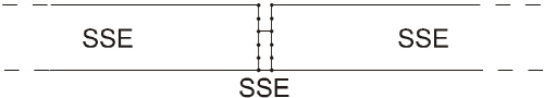
If a local non-uniformity has a uniform cross-section along its short length, it could be replaced by another SSE, rather than using a FE. A schematic diagram for this modified attempt is illustrated in Fig. 1(a).

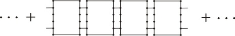
One further application of the combined SSEs would be waveguides with periodic non-uniformities, as illustrated in Fig. 1(d), such as periodically ribbed or supported plate or cylinders, etc. There are several papers in literature on theoretical analysis for wave propagation along periodic beam structures,^[12-14] but a little has found about plates.^[15] In the present study, wave propagation through the periodically stiffened plate is newly attempted by using the Floquet’s principle and the SSEs.

In the present paper, the combined SSEs are applied for two examples:a folded beam with an offset and a periodically ribbed plate. The first example is to check the validity of the proposed method with a simple beam model The second example is an expanded application of the presented approach for periodic structures. By using the periodic structure theory, the features of the pass- and stop-bands are investigated from this ribbed plate example.

II. Wavenumber domain finite element modeling

2.1 WFE equations

For infinite or finite length waveguides with homogeneous cross-sections, wavenumber domain finite element method ^[9-11] can be used effectively to investigate sustained wave types and their dispersion relations. The governing WFE equations are briefly described in this section. Refer to references 9-11 for more details.

Suppose that there is an elastic waveguide structure which is infinitely long in one direction, call it the -direction, and its cross-section normal to the x-axis is uniform along . The WFE governing equation is given by

where , and are stiffness matrices, is the mass matrix of the cross-section and is the cross- sectional displacement vector.

In the present study, all the wave solutions, including nearfield waves, are required to predict displacement of the waveguide with local non-uniformities. Hence Eq. (1) has to be solved as a polynomial eigenvalue problem about for given frequencies. Note that Eq.(3) will have paired wavenumber solutions, representing the positive- and negative-going waves at each frequency. For example, for a cross-sectional model with N dofs, 2N wavenumbers and mode shapes will be obtained at each .

The displacement of a finite and semi-infinite length waveguide structure can be written as a superposition of each wave solution obtained from Eq.(1). The displace-ment vector at frequency can be written as

where is a matrix containing each wave's mode shapes, is a diagonal matrix containing the exponential terms for and the subscript ‘’ represents variables for the positive-or negative-going waves along the x-direction, respectively. In Eqs. (2) and (3), corresponds to the wave amplitude vector.

If an input force vector, , is specified at the boundaries of the finite or semi-infinite waveguide structures, the displacement vector at the boundaries can be calculated using a dynamic stiffness matrix of the structure.^[16] Equations for and refer to reference 8. in detail. Hence, if an input force vector is given, the nodal displacement can be found using a dynamic stiffness matrix of the structure by

2.2 Combined models

Combined model is built by connecting dynamic stiffness matrices for each segment. Suppose there is a local discontinuity in the middle of an infinite length waveguide as illustrated in Fig. 1(a). This system can be divided into three parts; two semi-infinite SSEs and a finite SSE. To couple the semi-infinite SSEs with a finite SSE having a reduced cross-section, the dynamic stiffness matrices of them (, and in order) need to be combined. In case of semi-infinite waveguides with dofs, the sizes of and become . For the finite SSE with dofs, has the size of .

 The size of the combined dynamic stiffness will be determined by the largest dofs in the model. If , the combined dynamic stiffness of the connected SSEs will have a size of , given by

where 

In Eq. (6), and are submatrices of , which will be connected to the semi-infinite SSEs at the left-hand right-hand boundaries, respectively. If external force vector of size is established for each dofs on the boundaries, the displacement vector at the boundaries can be determined from and as given in Eq. (4).

For periodic waveguides as illustrated in Fig. 1(b), a dynamic stiffness of a repeated unit segment is required. Considering that two SSEs compose a repeated segment, it may be given by Eq. (14),

where and denotes the dynamic stiffnesses of the elements which consist of the repeated unit segment and the subscripts L and R correspond to the ‘left’ and ‘right’ boundaries of the unit segment.

Since this unit segment is repeated along the x direction, the Floquet’s theorem can used as given by

where is the transfer matrix and is the propagating constant which is generally complex, representing amplitude and phase change, i.e., over a single segment. and are called the attenuation constant and phase constant, respectively.

Eq. (8) is in the form of eigenvalue problem. However, the transfer matrix is likely to be ill-conditioned because the eigenvector is composed by displacements which are quite small and forces which are quite large, relatively. To improve the conditioning of the eigenvalue problem, Zhong’s method^[14] is introduced to obtain propagating constant reliably in this study. The details of Zhong’s method can be found in the references 17,18.

The reformulated eigenvalue problem by the Zhong’s method is given by

where the eigenvalue and

From the eigenvalue of Eq. (9), the propagation constants of each wave are calculated, which reveal their stop- and pass-band features.

Using Eqs. (7) and (8) from combined SSEs, the propagating features of waves in periodically non-uniform waveguides can be dealt with relatively easily, compare to the conventional FE approach.

III. Examples

The combined SSE method described in the previous section is applied to two examples in this section; connected beams with an offset and a rail with a sawcut-like defect. For these two examples, the power reflection and trans-mission coefficients are calculated, which are caused by the local non-uniformities. Also the numerical errors of the presented method are evaluated in terms of the incident power conservation in order to justify the combined SSE method.

3.1 Rail with a defect

For a rail with a simple sawcut-like defect growing from the top of the rail head, power reflection and transmission coefficients have been previously investigated in the references 8. by using a combined SSE/FE method. In that calculation, the combined SSE/FE method took several hours to obtain the results for a size of the defect. The main reason of the long time spending was due to the inversion of the FE matrices which are large in size. So if the FE part is able to be replaced by SSE, the computational burden would be much diminished.

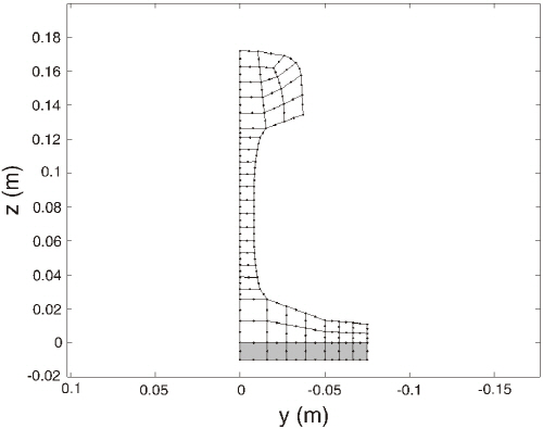
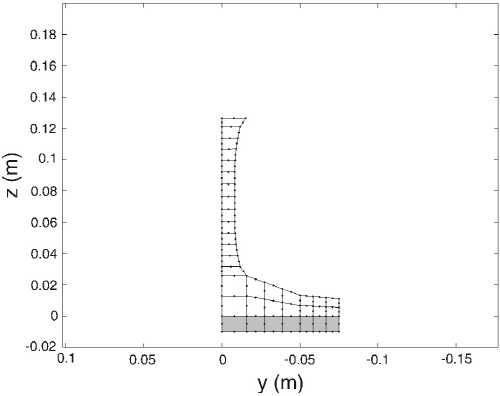
The cross-sectional models of the rail (UIC60) are shown in Fig. 2 for the homogeneous and defected parts. Since the UIC60 rail has a symmetric cross-section, only half of the width is modeled. In this example, a sawcut-like defect in the rail head shown in Fig. 2(b) is considered, which has 6 mm in length in the x-direction. Dispersion curves for the homogeneous rail shown in Fig. 2(a) are reported in the reference 19.

A technique imposing incident waves to the combined SSE method is the same as those for the combined SSE/FE approach described in the reference 8. For an incident wave indexed j, the power reflection and transmission coefficients for the ith reflected and transmitted waves are defined by

where and denote power reflection and transmission coefficients respectively, denote powers of traveling waves. The power reflection and transmission coefficients are calculated up to 40 kHz for the vertical bending wave in the railhead as an incident, reflected and transmitted waves of interest. The coefficients predicted by the combined SSE method are illustrated in Fig. 3. Fig. 3 shows that the vertical bending wave in the rail head has relatively large reflection in between 17 and 30 kHz while the large transmission in between 10 and 15 kHz. This feature of the chosen wave against frequency agrees well with the wave mode conversion phenomenon called curve veering.

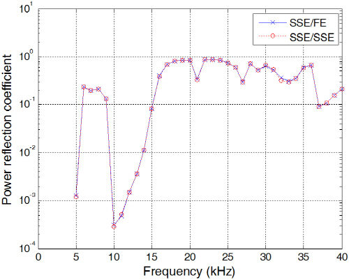
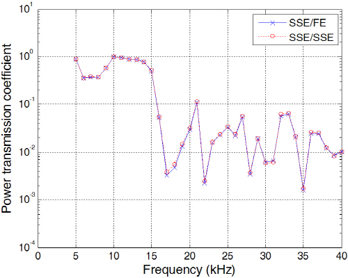
The results obtained from the combined SSE method are also compared in Fig. 3 with those from the combined SSE/FE method. It can be seen from Fig. 3 that the two methods create almost the same results in whole frequency range but the computational demand of the former is much less than that of the latter. The combined SSE method has taken a couple of minutes to get the result in Fig. 3 while the combined SSE/FE method has spent several hours to obtain the same results.

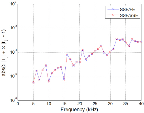
The incident power should be conserved if there is no damping in the model. That is, the reflected and transmitted waves should satisfy the condition

Using Eq.(12), the numerical errors predicted from the combined SSE model and SSE/FE model are illustrated in Fig. 4 in terms of the power conservation. It was found from Fig. 4 that both methods possess nearly the same errors which are low enough compare to the predicted reflection and transmission coefficients. Therefore, it can be surely said from this example that the combined SSE method is more efficient than the combined SSE/FE method, particularly for complex waveguides at high frequencies.

3.2 Periodically ribbed plate strip

A plate strip simply supported at both edges is regarded in this example as illustrated in Fig. 5. The plate was set to have a width of 0.5 m, thickness of 2 mm. Detail properties of the plate and ribs are listed in Table 1. The ribs are attached on the plate surface with a period of 0.2 m along the direction as shown in Fig. 5. The strip plate and rib were modelled with respective 10 and 20 solid elements and the dofs of 153 and 249 in total, respectively.

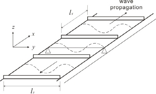
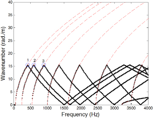
Before applying the combined SSE/SSE method to the ribbed plate, the dispersion curves for homogeneous strip plate predicted by Eq. (9) is compared in Fig. 6 with those obtained from the WFE method by Eq.(1) to validate the SSE/SSE method. These two results must be identical because the ribs are not involved in this calculation. It is obviously seen in Fig. 6 that they are the same except the SSE/SSE results are bounded from 0 to , which is decided by the length of the periodic segment. From the results in Fig. 6, it was validated that the SSE/SSE method is reliable.

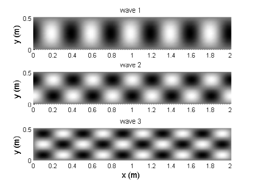
For the first three waves marked with circles in Fig. 6, their deformation shapes are shown in Fig. 7, corresponding to the waves having the first, second and the third cross-sectional modes along the y axis. When , odd multiples of the half wavelength are placed within .

On the other hand, when , even multiples of the half wavelength occurs within the period . Discussion for the bounding frequencies, where the wavenumbers are 0 or , is presented in the reference 20 in terms of the deformation of the periodic unit segment.

The bounding frequencies form pass- and stop- bandscharacteristics of periodic waveguides. For homo-geneous plates, all frequencies correspond to pass-band because there are no local non-uniformities along its length. However, a waveguide with a periodic non-uniformity, such as a ribbed plate, will have pass- and stop-band features at bounding frequencies.

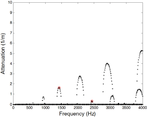
Fig. 8 shows the dispersion relations and decaying features of each wave propagating along the periodically ribbed plate strip, listed in Table 1. Figs. 8(a) and 8(b) come from the phase constant () and attenuation constant () divided by , solving Eq. (16). It can be seen from Fig. 8 that the attenuation occurs at frequencies where and and grow for higher order waves. The frequency bands where the attenuation occurs are called stop-band and the rest are pass-band, where waves can travel without decaying due to the periodic ribs. Meanwhile within a same single wave, for example, the fourth wave with circular marks in Fig. 8, the attenuation reduces as frequency increases. This shows that the ribs are acting as added stiffness which affects more at low frequencies.

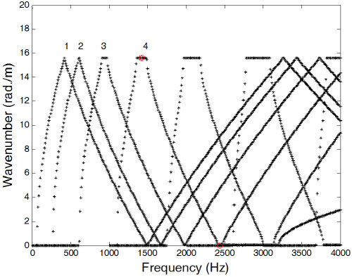
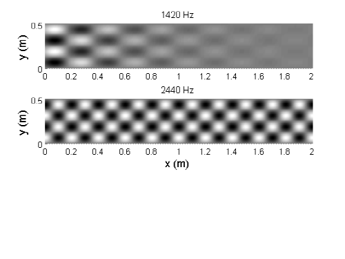
Deformation shapes of the ribbed plate generated by the fourth wave are displayed in Fig. 9 at two different frequencies marked with circles in Fig. 8. It can be seen from Fig. 9 that the wave decays along the x axis in their stop-bands.

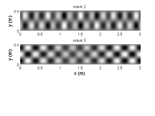
Since the attenuation at 1420 Hz is much higher than that at 2440 Hz, the wave at 1420 Hz decays more rapidly. On the other hand, waves 2 and 3 propagating within their pass-bands are illustrated in Fig. 10at 1 kHz. The deformation patterns in Fig. 11 shows that the waves travel along the x direction with amplitudes modulated or enveloped.

V. Conclusions

In this paper, wave propagation along waveguides with local or periodic non-uniformities was investigated by combining SSEs. Non-uniformities which have uniform cross-sections along their lengths were modeled by SSEs, instead of FEs. So, in the present study, the combined SSE/FE method was improved by replacing the FE part with a SSE and named it a combined SSE method.

Two examples, a rail with a sawcut-like defect and a periodically ribbed plate, were investigated in the present paper. For the first example, the power reflection and transmission coefficients were predicted, caused by the local non-uniformities. From this application, it was found that the errors of the combined SSE method are fairly small and almost identical to those of the combined SSE/FE method.

In the second example, a periodic structure theory was introduced and used together with the combined SSE method to predict wave propagation along periodically non-uniform waveguides. From this example, the pass- and stop-band characteristics of the ribbed strip plate were obtained by using a periodic structure theory and dynamics stiffness matrix generated by the combined SSE method. As the further application, the same approach is going to be applied to the ribbed cylinders and then attempted to couple external fluids.