I. Introduction

The official name of the ‘Formula One’ (or ‘Formula 1’ (or ‘F1’ in short)) is an acronym for ‘FIA Formula One World Championship’ and refers to the car racing, which is administered by the organization of ‘Fédération Internationale de l’Automobile (FIA). Here, ‘Formula’ means a set of requirements for the car (called machine) to satisfy.[1]

Historically, the earliest racing is traced back to 1920 when the ‘Grand Prix Motor Racing’ was held in Europe.[2] However, it is acknowledged that the first official formula was set up in 1946 and the first racing was held in 1947. Next, the worldwide championship was first open in 1950’ Silverstone racing in England and is continued up to date.

The winner is determined in a peculiar way. Only 24 racers are entitled to drive the machine and the 12 teams composed of them do the racing all around the world. The team of the highest accumulated score wins the championship.

A fancy expression of the marvelous feature for the F1 racing is “watch the sound!” which is spoken by a specialist in this field. The roaring and thundering sounds of the competing machines are impressive and unforgettable.

While the attractive feature of the tolling bell is in its beats, the wonderful aspect of the F1 sounds is in the Doppler effect: the pitch decreases dramatically as the machine bypasses the listener. Along with this frequency shift, the acoustic level change is accompanied as the machine approaches and recedes away. Considering the speed of the machines, all the changes occur in a very short time interval and the effect is as much drastic.

Organization of this paper is as follows. In section II, the Doppler effect will be reviewed for a general case in the sense that the listener is away from the rectilinear path of the machine’s motion. In section III, numerical investigations will be performed to draw expressions of the frequency as functions of time and the machine location. It will be revealed that a sigmoid function of tanh is reasonably good. After providing an application of the developed theory in this paper to the actual F1 machine’s sound in section IV, concluding remarks will be given in section V finally. Table 1 is the list of the variables and their meanings that will be used in this paper.

II. The Doppler Effect

 Though the stereo sound with two channels is more realistic and enriching, we will consider one-channel mono sound for the sake of simplicity of theoretical analysis. Fig. 1 shows an arrangement where a listener is located at a point

on the axis and the F1 machine is moving along the axis at a constant speed while generating a sound of peak frequency .

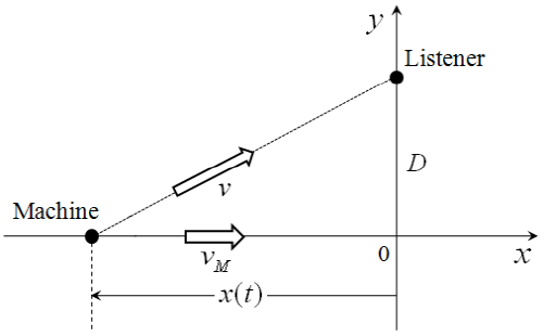
It is worth of note that the speed of sound, , is independent of the motion of the sound source. Instead, it is determined in terms of the physical properties of the medium, i.e. air, and its value is about 340 m/s at atmospheric pressure and temperature of 15℃.[3]

At time , the coordinate of the machine is given by

where is the its initial position. We divide this equation by to obtain

where the following quantities were defined:

These ‘scaled’ (dimensionless) variables allow us to extract results that are independent of the specific values of the distance and the frequency . At time , the distance from the listener to the machine is given by

where is the machine-to-listener distance.

At times

the machine is located at

and emits the -th wavefront. At those discrete times given by (1), the machine-to-listener distance is

The time of travel of the -th wavefront from the machine to the listener is given by

where a parameter

 was defined. The time at which the listener senses the -th wavefront is then given by the sum of (1) and (2):

The frequency of the sound felt by the listener is given by the inverse of the time interval of the consecutive wavefronts:

At the instant the listener senses this frequency, the machine is located at

where the ratio

denotes the machine’s Mach number.

Eq. (5) tells that, at the instant the listener senses the -th wavefront, the machine is located at the position advanced by from the position of the emission of the -th wavefront. Fig. 2 shows the frequency felt by the listener [Eq. (4)] vs. the location of the machine at the instant when the listener senses that frequency [Eq. (5)]. The Mach number was taken to be , which corresponds roughly to . The overall feature ofFig. 2 is in qualitative agreement with the work of Lee and Wang.[4]

For the wavefront that the machine emits at the position , the listener does not feel frequency shift and thus senses the frequency and, at that moment of sensing that wavefront, the machine is located at the position , the coordinate of which is marked by a dot in the graph.

The two frequencies

denote the cases of the longitudinal Doppler shifts () for the machine to approach towards [Eq. (6)] and recede away from [Eq. (7)] the listener, respectively.[5] In this case, the frequency perceived by the listener shows abrupt change from to as the sound source passes by him. This case differs from Fig. 2 in that the shape of the frequency change is given by a Heaviside (step) function, rather than a graded one.

The other two dotted lines in Fig. 2 represent the frequency of the machine

and the arithmetic mean of and , i.e.,

III. Curve-Fitting by a Sigmoid

The curve of Fig. 2 has the shape of a graded step function which is antisymmetric with respect to and converges towards two extreme values at both ends. To represent this curve by a sigmoid function, we consider

where and are adjustable parameters for the best fit. can be fixed from the constraint

and we] get

To obtain , we consider an objective function

where and are given by Eqs. (4) and (5), respectively. is then determined by

Fig. 3 shows the objective function vs. the parameter for . It decreases as , reaches the minimum, and then grows.

The value of for the best fit depends on . Fig. 4 shows the result. A curve-fitting by a second order polynomial gives

Collecting the results, Eq. (8) might be written as

which represents the frequency felt by the listener as a function of the machine’s location at the instant of frequency sensing. This expression is notable in that it includes only one parameter . Fig. 5 is an example of the curve-fitting by Eq. (9) for .

Fig. 6 shows the same result as Fig. 5 with the physical values of and , the standard tuning frequency, instead of scaled ones.

The frequency felt by the listener vs. the time of frequency sensing, i.e. Eq. (4) vs. Eq. (3), is plotted in Fig. 7. It has also the shape of a graded step function.

Similarly to Eq. (9), we try modelling of this curve by

where is a parameter to be adjusted for the best fit and is the time when the frequency has the value . Fig. 8 shows the curve-fitting result for .

We see that the frequency felt by the listener vs. the time of frequency sensing might also be represented by the tanh function reasonably well. A universal expression for such as (9) is not allowed due to unavailability of the general expression for the time and thus it will not be pursued further in this paper.

IV. Analysis for an Actual F1 Sound

Fig. 9 shows a part of the sound of the Ferrari machine in the ‘2009 FIA WTCC Race of Italy’.[6]

Fig. 10 is an enlarged view of the section ‘A’ of Fig. 9. The number of data points is 1,024 for FFT and the time duration is 64ms. Fig. 11 is the FFT for the data of Fig. 10.

For most of the analysis frames consisting of 1,024 data points, the peak frequency (PF) can be identified clearly as in Fig. 11. However, it is not always the case. Fig. 12 and Fig. 13 show the FFT results for the sections of ‘B’ and ‘C’ of Fig. 9.

The PFs may come from other sources than the engine. For an example, noises from muffler, tire, and wind might intervene the F1 sound of our interest.[7] If these are the cases, separation of the sound sources might be useful by independent component analysis.[8]

The PFs of Fig. 12 and Fig. 13 correspond to the third and second harmonics of Fig. 11, respectively, with some minor numerical deviation. It is not easy, though not impossible, to set up a numerical criterion for treatment of these harmonics in an automatic fashion.

Fig. 14 shows PF profile for Fig. 9 in continuous manner by picking up the PF for each analysis frame consisting of 1,024 data points.

The overall feature shows a graded step function with some undesirable pulse-like peaks coming from harmonics. These unwanted peaks might be corrected by identifying the harmonics, but we discard the undesirable high frequency peaks above 1 kHz. The result is shown in Fig. 15. We see that the overall feature is similar to Fig. 8.

The extreme values of the frequency on the left and right side were estimated to be

By applying Eqs. (6) and (7) to these values, we obtain

To compare experimental data with the theory developed in this paper, we try to fit the data of Fig. 15 by a sigmoid function

with two adjustable parameters and . From Eq. (11), we have and is estimated to be

from the condition

Adjustment of is done by the least-square scheme as before, the result being

Fig. 16 shows the result.

We see that the experimental data is in reasonable agreement with the theoretical fit. All in all, the frequency sensed by a listener a distance away from the path of rectilinear movement of the sound source might be represented by a sigmoid function.

V. Conclusions

In this paper, we analyzed the sound generated from F1 machine by the Doppler effect. For the case the listener is away from the rectilinear path of the F1 motion, the frequency shift felt by him was derived as functions of time and machine location. The result was found to be graded step function. From numerical analyses, it was shown that the function was described by tanh sigmoid function reasonably well.

In order to apply the theory to the actual F1 machine sound, FFT (Fast Fourier Transform) was performed on the Ferrari engine sound. The peak frequencies were estimated with exclusion of the high frequency harmonics. From the two asymptotic frequencies for approaching and receding cases, the intrinsic frequency of the engine and the speed of the machine were obtained.