

I. Introduction
II. General linearly constrained broadband adaptive array
III. General adaptive algorithm
IV. Simulation results
V. Conclusions
I. Introduction
The linearly constrained adaptive arrays[1,2] depends on the extent of the correlatedness of the desired signal and the interference signals. If the desired signal is partially or totally correlated with the interference signals, the desired signal is partially or totally cancelled in the array output. A variety of algorithms were proposed to reduce the signal cancellation phenomena.[2-8]
In this paper, a general linearly constrained adaptive array is proposed to improve the nulling performance. The nulling performance is examined in the array weight vector space. It is assumed that the direction of the desired signal is known a priori. The error output is generated by the array output subtracted by the desired response which is formed as the output of the multichannel uniform all-pass filter weighted by a gain factor.
The linearly constrained broadband adaptive array is implemented in coherent and noncoherent signal environmen-ts. It is shown that the value of the gain factor affects the nulling performance such that there exists a value of the gain factor which yields a best nulling performance.
Adaptive Array processing techniques have been applied in many areas which include radar,[9] sonar,[10] and seismology.[11]
II. General linearly constrained broadband adaptive array
In the conventional linearly constrained adaptive array[1] proposed by Frost, it is assumed that the desired signal is uncorrelated with the interference signals. If the desired signal is correlated with the interferences, it is demonstrated that the desired signal is cancelled in the array output.[2]
A general linearly constrained adaptive array is proposed to reduce the signal cancellation phenomena in coherent and noncoherent signal environments. The general linearly constrained broadband adaptive array with N sensor elements followed by L taps per element is shown in Fig. 1.
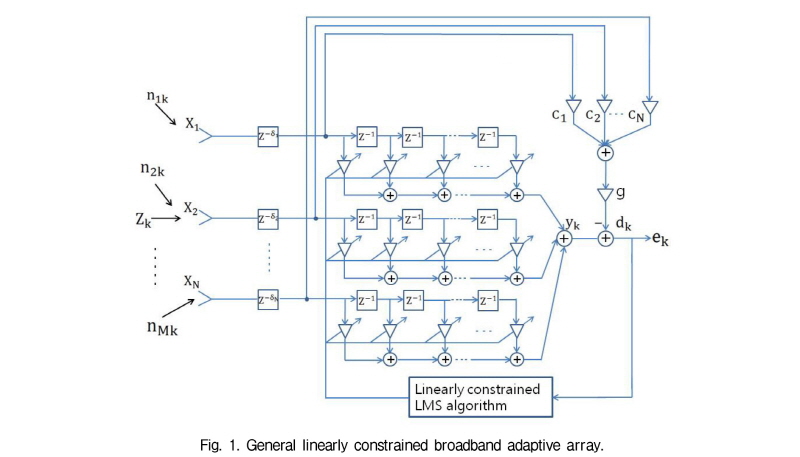
The desired signals at each channel are delayed after they pass through the steering time delay elements right after the each sensor such that the desired signal becomes in phase after the steering time delay elements. The desired response is generated by multiplying the output of the multichannel uniform allpass filter (i.e., all weights zero except for the first column of uniform weights) by a gain factor.
The optimum weight vector which yields a minimum mean square error output with a unit gain constraint at the look direction (i.e., the direction of the desired signal) can be found by solving the following constrained optimization problem.
min 
subject to  , (1)
, (1)
where an  weight vector
  , the
, the  weight vector
  of the multichannel allpass filter
is given by  in the figure,
 , 1<i<N. R is an NL×NL input signal correlation
matrix, which is given by  and the input signal vector
  . The
. The  th column vector of the
  constraint matrix
  consists of elements of 0 except of the
  th group of
  elements of 1, and the
  constraint vector is given by

The optimum weight vector can be found by the method of Lagrange multipliers solving the unconstrained optimization problem with the following objective function.
 , (2)
, (2)
where  is a
is a  Lagrange multiplier vector. The gradient of the objective function is given by
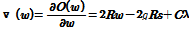 . (3)
. (3)
By setting the gradient equal to zero, we have the optimum weight vector as
 , (4)
, (4)
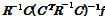
where  is
is  .
.
The optimum weight vector is obtained by finding  using the linear constraint in (1), substituting the resulting
 for that in (4). Then the optimum weight vector is given by

 . (5)
. (5)
The optimum weight vector in (5) could be interpreted geometrically in the translated weight vector space. If we denote the translated weight vector  as
as  , the optimization problem in the translated weight vector space can be formulated as
min 
subject to  . (6)
. (6)
The objective function with the Lagrange multiplier vector is represented as
 . (7)
. (7)
The optimum weight vector using the gradient of  is expressed as
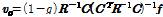 . (8)
. (8)
From (8), it is observed in the translated weight vector space that the constraint plane is shifted to the origin perpendicularly by the gain factor  such that the increase of the gain factor results in the decrease of the distance from the constraint plane to the origin. Thus the variation of the gain factor has an effect on the extent of orthogonality between the weight vector and the steering vectors for the interferences such that the nulling performance of the general linearly constrained adaptive array may be improved by the gain factor compared to the conventional linearly constrained adaptive array.
III. General adaptive algorithm
The general linearly constrained adaptive algorithm is derived by minimizing the mean square error using the steepest descent method.[12]
 , (9)
, (9)
where  is a convergence parameter and
  is a iteration index. Substituting the gradient in (3) for that in (9), we have the following iterative equation.
 . (10)
We find the Lagrange multiplier vector  by applying the
  th weight vector
  to the linear constraint in (1) to find the
  and substituting the
  for that in (10), we have the following general linearly constrained adaptive algorithm.
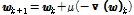
 , (11)
where the  projection matrix
  is given by
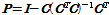 . (12)
which projects a vector onto the constraint subspace which is the orthogonal complement of the column space of  and the
  vector
  is given by
 . (13)
which is in the column space of  and normal to the constraint subspace.
A general linearly constrained LMS (Least Mean Square) algorithm can be obtained by substituting a instantaneous correlation matrix  for
for  in (11) and rearranging the resulting equation. Then the general linearly constrained LMS algorithm is expressed as
 , (14)
where  is the output error signal.
The array weights are updated iteratively by the general linearly constrained LMS algorithm in the computer sim-ulation.
IV. Simulation results
The linearly constrained broadband adaptive array with 5 sensor elements and 3 weights per element is employed to demonstrate the nulling performance of the general linearly constrained adaptive array. It is assumed that the incoming signals are plain waves. The incoming signals are generated by passing a white Gaussian random signal through the 4 th-order Butterworth filter such that the bandwidth is 3 Hz with the lower and upper cutoff frequencies 8 Hz and 11 Hz respectively. The sampling frequency is 608 Hz. The convergence parameter is assumed to be 0.0001.
The gain factor is varied to improve the nulling performance in coherent and nocoherent signal environments. The simulation results in[6] are redisplayed to demonstrate the nulling performance.
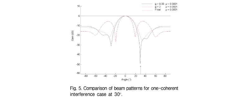
4.1 Case for one coherent interference
It is assummed that a coherent interference is incident at 30° with respect to the array normal. The variation of the error power between the array output and the desired signal is displayed in Fig. 2. The optimum value of is shown to be 0.33. The comparison of the array performance for  , the conventional linearly constrained adaptive array proposed by Frost and the case for
  are shown in Figs. 3 and 4 with respect to the array output and the desired signal for
  and
and  .
.
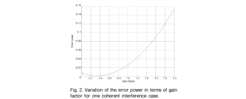
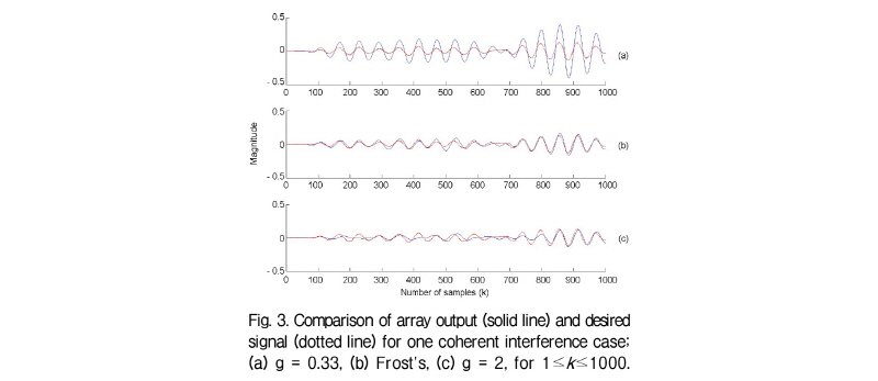
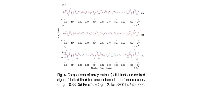
It is shown for  that the case for
  performs best while the Frost’s performs better than the case for
  . The beam patterns are shown in Fig. 5, in which the case for
  forms a deepest null.
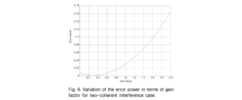
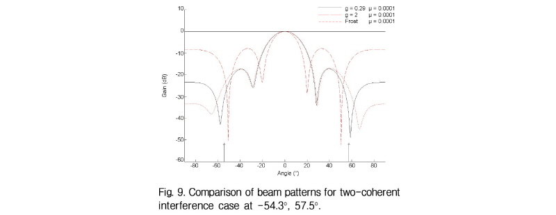
4.2 Case for two coherent interferences
It is assummed that two coherent interferences are incident at -54.3° and 57.5°. The variation of the error power between the array output and the desired signal is displayed in Fig. 6. The optimum value of  is shown to be 0.29. The compari-son of the array performance for
  . the conventional linearly constrained adaptive array proposed by Frost, and the case for
  are shown in Figs. 7 and 8 with respect to the array output and the desired signal for
  and
and  .
.
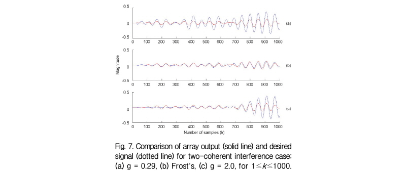

It is shown for  that the case for
  performs best while Frost’s performs better than the case for
  The beam patterns are shown in Fig. 9, in which the case for
  forms two deepest nulls around the two incident angles -54.3° and 57.5° of the coherent interferences.
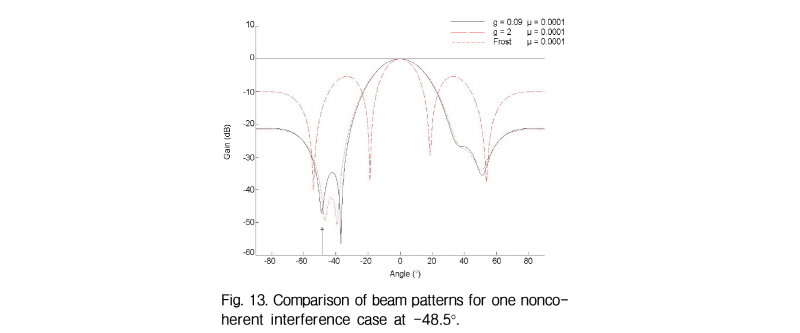
4.3 Case for one noncoherent interference
It is assummed that a noncoherent interference is incident at -48.5°. The variation of the error power between the array output and the desired signal is displayed in Fig. 10. The optimum value of  is shown to be 0.09. The comparison of the array performance for
  , the conventional linearly constrained adaptive array proposed by Frost, and the case for
  are shown in Figs. 11 and 12 with respect to the array output and the desired signal for
  and
and  .
.
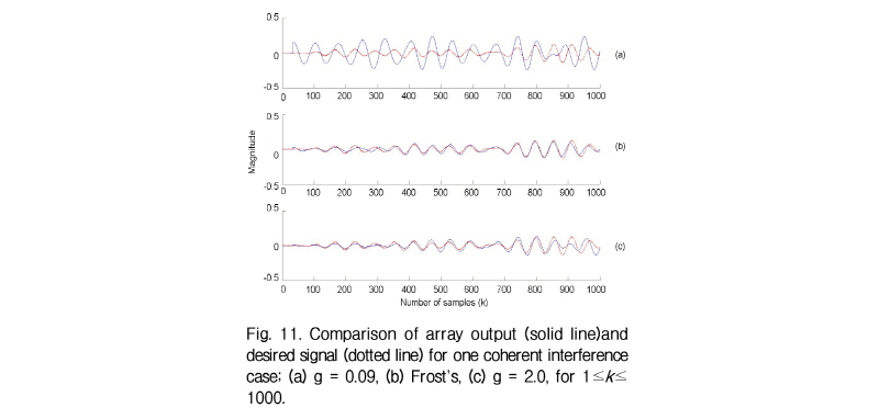
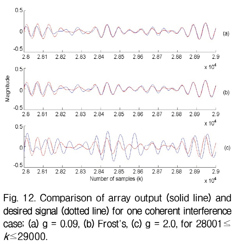
It is shown for  that the case for
  and the Frost’s array yield a similar performance while both of them performs better than the case for
  . The beam patterns are shown in Fig. 13, in which the case for
  and the Frost’s array yields a similar gain at the incident angle of the noncoherent interference. It is observed that a more exact null is formed at the incident angle of the noncoherent interference for the case of
  than for the Frost’s.
V. Conclusions
A general linearly constrained adaptive array is proposed to improve the nulling performance in coherent and noncoherent signal environments. The nulling perfor-mance is examined in the array weight vector space. It is observed that the constraint plane is shifted to the origin perpendicularly by the value of the gain factor such that the increase of the gain factor results in the decrease of the distance from the constraint plane to the origin.
Thus the variation of the gain factor has an effect on the extent of orthogonality between the weight vector and the steering vectors for the interference signals such that the orthogonality between the weight vector and the steering vectors for the interference signals is improved at an optimum gain factor. Therefore, the nulling performance of the general linearly constrained adaptive array with an optimum gain factor is improved compared to the conventional linearly constrained adaptive array.
It is demonstrated in the computer simulation that the general linearly constrained adaptive array performs better at the optimal gain factor than the conventional linearly constrained adaptive array in coherent environment while it yields a similar performance to the conventional linearly constrained adaptive array in noncoherent environment.
