

I. Introduction
II. Proposed Method
2.1 Feature Extraction
2.2 ALexNet
III. Experimental Work
3.1 Dataset
3.2 Experimental Setting
3.3 Results and Discussion
IV. Conclusions
I. Introduction
Recently with the rapid development of AI (Artificial Intelligence), environmental sound classification has been a research focus of many applications from surveillance,[1] to environmental monitoring.[2-5] AI has been applied to the detection and classification of certain animal species through acoustic sounds to provide information used by applications monitoring biodiversity and endangered species preservation. These environmental monitoring applications classify the sounds of animals ranging from marine life[3,4] to bats[5] or birds.[6,7]
To capture the information contained in acoustic event classification,[8,9] sound and automatic speech recognition[10–12] have used several features, such Mel-log filter bank and MFCCs (Mel Frequency Cepstral Coefficients), which are based on the human auditory system. Even though such features have dominated in acoustic applications, and continue to do so, their performance decreases with the amount of noise present in the signal. Therefore, several attempts to suppress noise without distorting the acoustic signal have been proposed using stationary noise suppression mechanisms to achieve system performance under environmental noisy conditions. These methods include the use of the Wiener filter, PNCCs (Power Normalized Cepstral Coefficients)[13] and RCGCCs (Robust Compressive Gamma-chirp filter bank Cepstral Coefficients).[14] While such features do improve performance, their effectiveness still depends on the types or characteristics of the noise present, such as whether it is non-stationary noise. Interestingly, recent research has shown that using combinations of features can boost overall system performance. For example, References [15], [16] show that combining MFCC features with PNCC features, which are both robust to noise, makes the overall system, which can then learn from and exploit both features, perform better under noisy environments.
In this work, we investigate combined robust feature performance under noisy environments using both PNCCs, and the log Mel-filter bank integrated with the Wiener filter, which both work with stationary noise but use different stationary noise suppression algorithms. Firstly, the Wiener filter is combined with the log Mel-filter bank to suppress stationary noise which is an optimal causal system where the power spectrum of the noise is estimated based on the present and previous signal frames to provide an estimate of the clean signal based on the mean square error. Integrating the Wiener filter will allow use of a log Mel-filter bank and also suppress noise using an optimal estimation.[17] Secondly, the PNCCs are employed as they achieve good performance under noisy environments by applying the medium duration power bias subtraction algorithm, which is based on asymmetric filtering and temporal masking effects. Additionally, the PNCC uses the power law nonlinearity with gammatone filter instead of the log and the triangular filter used by the log Mel-filter bank.[13] Given the different characteristics of these features, we expect that combining them through a convolutional layer that enables the system to extract features from both will boost system performance for bird sound classification under both clean and noisy environments. The proposed extraction method is explained in more detail in section II and the experimental work and discussion in section III.
II. Proposed Method
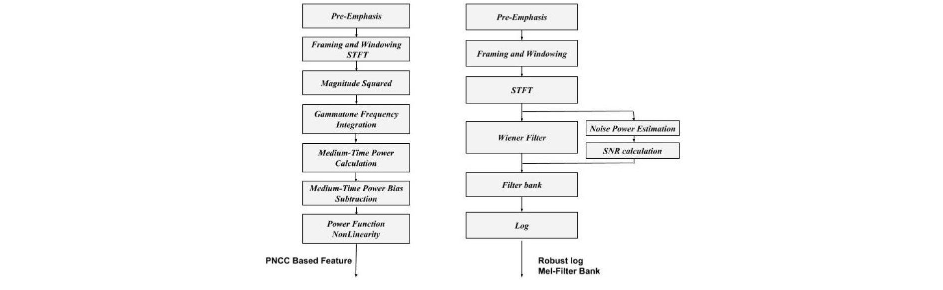
This section describes the proposed method consisting of two principal stages, the feature extraction stage and the classification stage, which uses the AlexNet structure[18] to classify bird species. In the feature extraction stage, both the log Mel filter bank with Wiener filter and PNCC noise estimations and their characteristics will be elucidated in more detail as well as the combining procedure of both features that feeds into the AlexNet network. Fig. 1 illustrates the feature extraction steps of both features.
2.1 Feature Extraction
2.1.1 Log Mel-Filter Bank with Wiener filter
Mel-filter bank is been widely used and it is designed based on the human auditory system. In order to extract the enhanced or robust features, the optimal Wiener filter is used after obtaining the spectrum of the signal following the work and recommendation in Reference [19]. As we assuming an additive noise as in Reference [20], where the Y(f), S(f), W(f) denotes the observed, desired, and noise signal in frequency domain. Also, the Wiener filter output or transfer function can be expressed in the frequency domain as in Eq. (2), clean or enhanced signal can be demonstrated using Eq. (3).
| $$Y(f)=S(f)+N(f).$$ | (1) |
| $$H_{wiener}(f)=\frac{P_{ss}(f)}{P_{ss}(f)+P_{nn}(f)}.$$ | (2) |
| $$P_{ss}(f)=H_{wiener}(f)\;P_{YY}(s).$$ | (3) |
The Pss and Pnn are the desired observed and noise power spectra, respectively. Therefore, the estimated signal can be obtained through Eq. (3) by first estimating the noise signal spectrum using the MMSE-SPP (Minimum Mean Square Eerror - soft Speech Presence Probability) algorithm proposed in Reference [21], which does not require bias correction or VAD (Voice Activity Detection) as the MMSE-based noise spectrum estimate approach would.
2.1.2 PNCCs (Power Normalized Cepstral Coefficients)
The PNCC features are designed for stationary noise suppression, a goal which can also be achieved using the log Mel-filter bank. However, the PNCC algorithm has three main differences. It uses the gammatone filter to replace the filter bank and applies power-law nonlinearity based on the hearing of Steven’s law power[22] as this approach leads to close to zero output when the input is too small, in contrast to the log function that is used for the Mel-log filter bank features. In addition, it performs a peak power normalization using the medium-time power bias subtraction method proposed in Reference[13]. This method does not estimate the noise power from non-speech frames, but instead removes the power bias that has information about the level of the background noise as assumed, and uses the ratio of the arithmetic mean to the geometric mean when determining the power bias. The final power can be obtained through Eqs. (4) - (6).
| $$Q(i,j)=\frac1{2M+1}\;\;\sum_{j'=j-M}^{j+M}\;P(i,j').$$ | (4) |
| $$Q'(i,j\left|B\right.(i))=\max(Q(i,j)-B(i),d_0Q(i,j)).$$ | (5) |
| $$\widetilde p(i,j)=\left(\frac1{2N+1}\;\sum_{i'=\max(1-N,1)}^{\min(i+N,C)}\;\frac{Q'(i,j\left|B(i))\right.}{Q(i,j)}\right)P(i,j).$$ | (6) |
Hence, i is the channel index, j is the frame index, C is total number of channels, P(i,j) is the power observed in a single analysis frame, Q(i,j) is the average power of 7 frames (M = 3), and the normalized power can be obtained by subtracting the level of background excitation (B(i) ). In addition, the d0 in (5) is constant to prevent the normalized power from becoming negative. Therefore, the final power ((i,j)) can be obtained though Eq. (6). For more details refer to Reference [13].
2.1.3 Features Combination using Convlutional Network
This stage aims to find the best feature representation of data based the available features map using the convolutional neural network. Where, the combined features are obtained by concatenated both extracted features and create a 3-dimensional features (features, frames, 2) in order to be fed into a convolutional layer to get only one feature mapping representation (k = 1) of both extracted feature type (features, frames, 1), whereas the mapping is done with a trainable filter size of (l, l, q) known as filter bank (W) that connect the feature map (q = 1) of the input to the layer into the output or desired map (k) which can be obtained using Eq. (7).
| $$z^s=\sum_{t=1}^q\;W_t^{k\ast}x_{s,t}^i+b_s,$$ | (7) |
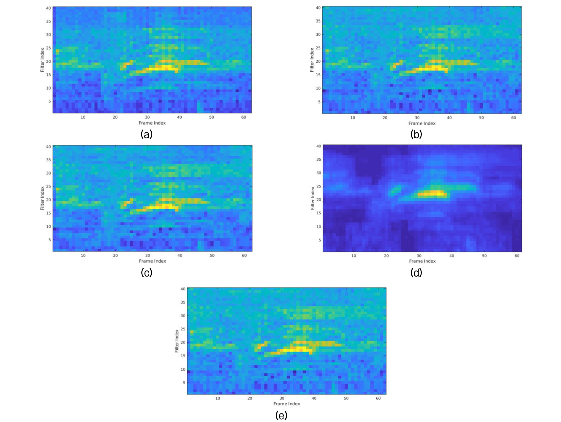
where * is 2-dim convolution operator, b is bias and denotes the features in each feature map.[23] This will allow the network to assign a certain weight or importance to each feature in the feature map for both the PNCCs and robust log Mel-filter bank. This leads to a better system performance by highlighting the most significant features that can post our system. Fig. 2 shows the power spectral density of the extracted features from the robust log Mel-filter bank, PNCCs and combined features under shop noise with an SNR (Signal to Noise Ratio) of 10 dB. Looking at the results we can observe that the combined extracted features seem to sum and exploit both features by keeping more information that are similar to the log Mel-filter bank and reducing a fraction of the added noise.
2.2 ALexNet
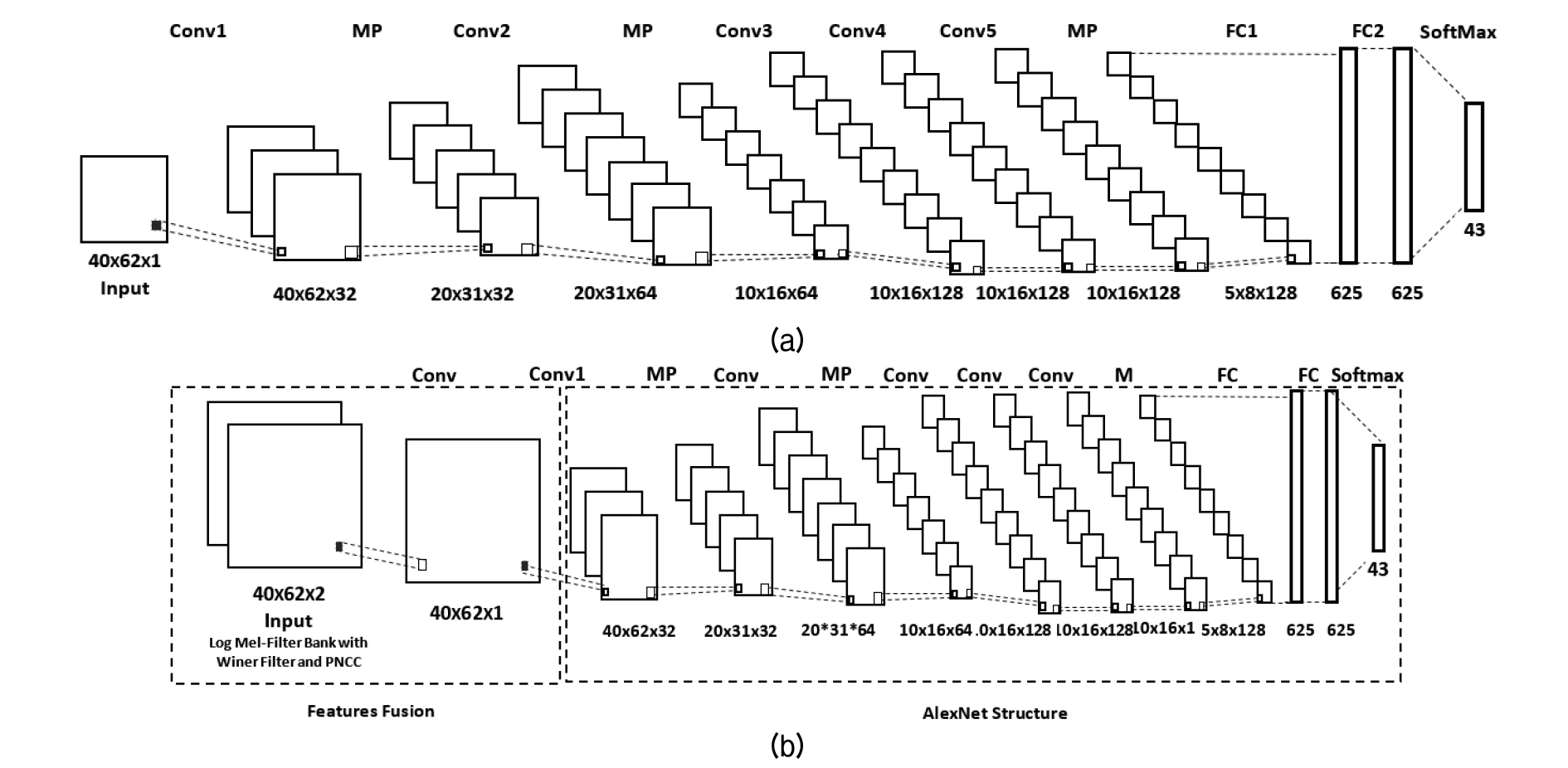
Based on References [18], [24], the CNN structure is composed of 5 convolutional layers with a 3 × 3 filter size and a stride of 1, and 3 max pooling layers. Max-pooling layers with a filter size of 2 × 2 and a stride of 2 were used after the first, second and the fifth convolutional layers. Three fully connected layers were used following the 5 convolutional layers separated by a dropout as used in References [24]. Fig. 3 illustrates the CNN structure for classification using the single feature and combined features.
III. Experimental Work
3.1 Dataset
The bird sounds were collected from https://ebird.org at a sample rate of 44.1 kHz, and down sampled to 16-bit resolution and segmented using the EPD (End-Point Detection) method[25] based on the procedure in Reference [7] for data processing and segmentation. This resulted in 0.719 s audio samples of 43 bird class species. The database was augmented with 3 types of background noise (café, shop and schoolyard) at 4 levels of SNR (20 dB, 10 dB, 5 dB and 0 dB) using ADDNOISE MATLAB.[26]
3.2 Experimental Setting
The baseline features are the log Mel-filter bank with and without the Wiener Filter, where the Wiener filter is applied after taking the spectrum of the signal, as well as the PNCCs. The features were extracted from 0.719 s audio sounds and resulted in 40 features with 62 frames per audio. These features were used as inputs to the AlexNet structure for classification as explained in Fig. 3(b). When using the proposed method, both the robust log Mel-filter bank (log Mel-filter bank with Wiener filter) and PNCCs were concatenated to get 3-D (40 × 62 × 2) arrays which were used as inputs to the network to extract one 3-D feature map, as explained in section 2 and illustrated in Fig. 3, using a filter size of (1, 1, 2). Moreover, the database was divided into training and test sets using 5-fold cross validation, resulting in 5 sets. Each feature vector was normalized by the mean and variance before being fed into the AlexNet for training. In the AlexNet structure, a dropout of 0.5 was used to reduce the effect of overfitting after the fully-connected layer, and ReLU (Rectified Linear Unit) activation function were used with batch size of 500.
3.3 Results and Discussion
Table 1 illustrates the overall accuracy for all 43 given classes for all 5 folds. The combined features gave the highest average accuracy of 82 % among all the features meaning an increase in average accuracy of 1.34 % over the Mel log-filter bank. This was followed by accuracies of 80.66 % and 79.46 % for the Mel log-filter bank and robust log Mel-filter bank, respectively. The PNCCs demonstrated the lowest average accuracy of 79.20 % with the clean data.
Table 1. Bird species classification in clean environment.
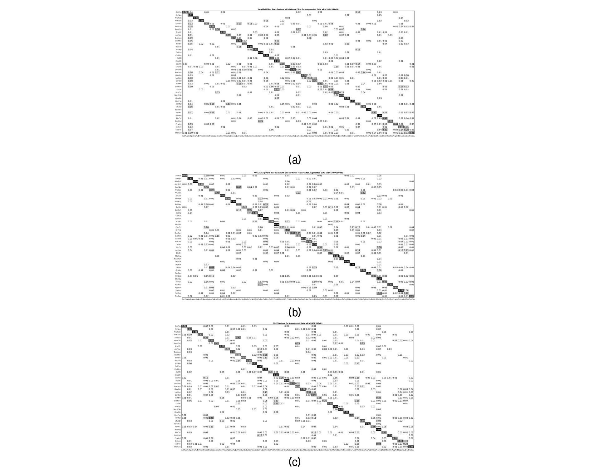
In addition, these features’ performances were tested on the augmented data and the results are presented in Table 2. Notably, the combined feature almost always outperforms the others except the cases of the café augmented data with SNRs of 5 dB and 0 dB where the PNCCs give the highest accuracy rates of 61.09 % and 48.85 %, respectively. The overall percentage increases in accuracy with shop and schoolyard background noise, respectively, under all SNRs were 1.06 % and 0.65 %. However, there was a decrease in average overall accuracy over all SNR levels for the café background noise type of 0.31 %. Fig. 4 shows the confusion matrix of the combined features, PNCCs and robust log Mel-filter bank under shop background noise with an SNR of 10 dB.
Table 2. Bird species classification accuracy in noisy environment.
However, the background noise is non-stationary noise and both features focus on a noise suppression feature that works with stationary noise. Therefore, the performance of the log Mel filter bank with the Wiener filter inevitably cannot give a better performance across all noise types and PNCCs enhanced the performance most effectively under the noisy environment. By combining these two features, the network seems to highlight and signify the most relevant features contained in both and therefore led to an increase in overall accuracy under both clean and noisy environments.
IV. Conclusions
In this work, we proposed 3-D combined robust features feeding to a convolutional layer followed by AlexNet for acoustic sound classification. The database of ebird.com was used to test the performance of the log Mel-filter bank, PNCC and combined features structure. The combined features structure outperformed the single features in most cases yielding an increase in accuracy by 1.34 % in a clean environment and 1.06 % and 0.65 % under shop and schoolyard background noise environments, respectively when averaged over 4 different SNR levels. These results illustrated that extracting these features from the combined ones using a convolutional neural network can exploit the complementarity of the combined features by making them accessible to the classification step, and thereby increase the recognition rate.
