

I. Introduction
II. Problem Statement
2.1 Binaural reproduction based on Ambisonics for virtual reality
2.2 Performance evaluation
III. Distortions of Binaural Sound Based on Ambisonics
3.1 Spectral distortions
3.2 ILDs and IPDs for a source located in the horizontal plane
IV. Discussions
4.1 Spectral compensation
4.2 Localization performance in the horizontal plane
4.3 The effect of the decoding methods
4.4 The effect of the layouts of loudspeakers
V. Conclusions
I. Introduction
Virtual Reality (VR) audio can be provided through headphones with binaural sound that compensates head rotation of a listener. One of the ways of obtaining the binaural sound is to convolute sound from sound objects and Head-Related Transfer Function (HRTF). This method is realizable only if positions of sound objects and their sound are known. In this case, sound localization and spectrum are not significantly distorted. However, ambient sound is hard to specify its position and sound because it is a mixture of several sound objects and their reflections. For ambient sound, therefore, another method is used: based on Ambisonics,[1] a sound field itself around the listener is recorded (encoding), the Ambisonic signals are converted to signals of virtual loudspeakers (decoding), and the loudspeaker signals and the corresponding HRTFs are convoluted to obtain the binaural sound.
Nevertheless, in physical point of view, the maximum cut off frequency for nearly perfect reproduction of HRTFs with Ambisonics is too low considering the audible frequency range. The maximum frequency can be calculated by the rule of thumb, ,[2], [3] where indicates the closest integer, N is the order of Ambisonics, kmax is the maximum wavenumber, and a is the radius of a listener’s head. For example, when assuming a is 9 cm, the maximum frequency with the first order Ambisonics (FOA, N = 1) is approximately 607 Hz. Above this frequency, impairments of spectrum and sound localization are unavoidable. This paper investigates these impairments by comparing the signals that arrive at ear positions in the reference and the reproduced fields. That is, a sound wave is assumed for a reference field, and this wave is reproduced with virtual loudspeakers based on FOA. The HRTFs in the reference field are compared with those in the reproduced field. Two Ambisonic decoding methods are used, the basic decoder based on the pseudo- inverse[2] and the maximum energy decoding (max RE),[3], [4], [5] which is known to improve the localization performance at high frequencies.
The HRTFs can be obtained by means of a rigid sphere model for a listener’s head as well as measurements. A listener’s head is sometimes modelled as a rigid sphere because sound pressure on its surface can analytically be calculated when an incident sound wave comes to a rigid sphere, and scattered.[6], [7] The rigid sphere model enables derivation of the ear signals in a closed form and also integration with respect to the incident angle of the sound wave. On the other hand, measured HRTF data show practical distortions, combined with other effects, e.g. shape of heads, torsos, and ears. Both of those HRTFs are used in this study: a rigid sphere model that regards the listener’s head a sphere of the radius 9 cm and a HRTF database of a dummy-head microphone.[8] Three loudspeaker layouts that have 4, 6, and 8 loudspeakers in uniform spacing (tetrahedron, octahedron, and cuboid, respectively) are employed for virtual loudspeakers. These layouts has been firstly considered in.[9]
Ambisonics has been proposed in 1970s by Gerzon,[1] and sound field microphones that are composed of 4 microphones in a tetrahedral layout have been also invented.[10] Ambisonics is theoretically based on the spherical harmonics expansion,[11] and the order of Ambisonics is defined by the maximum order of the expansion. FOA uses spherical harmonics expansion up to the first order. Higher-order Ambisonics (HOA), which has higher order than 1, have been proposed,[12], [13] and an array of microphones that are mounted on a rigid sphere have been invented that can acquire higher order components.[14] Several schemes of Mixed-order Ambisonics (MOA) have been also proposed that selectively use spherical harmonics components.[15], [16], [17] Recently, in connection with virtual reality applications, Ambisonics were widely used for immersive audio rendering, e.g..[18], [19]
Analyses on the Ambisonic reproduction have also been performed although not all these studies were based on the headphone reproduction.[20], [21], [22], [23] Solvang has shown that spectral impairments of Ambisonic reproduction,[20] but it was concerned with two-dimensional reproduction, and focused on the reproduced incident fields instead of the signals at ear positions. McKenzie et al.[21] analyzed the distortion of the spectrum, and proposed a diffuse-field equalization and a directional bias equalization.[22] These filters are based on a measured HRTF, and the frequency responses have a large deviation along the frequency. Satongar et al. investigated the localization performance of the first, second, and third Ambisonics by means of Inter-aural Level Differences (ILDs) and Inter-aural Time Differences (ITDs).[23] Both measured HRTFs and a rigid sphere were used for the investigation, but only horizontal loudspeakers were employed (2.5D reproduction). Localization performances of Ambisonics were subjectively investigated in listening tests,[24], [25], [26], [27] and distance and height perception with Ambisonics has been also analyzed.[28], [29], [30]
Spectral distortion with a rigid sphere model and localization performances with three-dimensional loudspeaker layouts have not been analyzed so far, and the decoding methods have not been compared in terms of ILDs and ITDs in previous studies. This paper analyzes distortions in terms of spectrum and sound localization, and considered several cases, i.e. two decoding methods and three loudspeaker layouts. Section 2 describes basic setup of this study, and Section 3 shows main results. Spectral compensation, the localization performance in the horizontal and the median planes, the effect of the decoding methods and the loudspeaker layouts are discussed in Section 4. Section 5 concludes this study. (Note that parts of this study has been presented in a conference.)[31]
II. Problem Statement
2.1 Binaural reproduction based on Ambisonics for virtual reality
In order to obtain the binaural sound, let us assume a single sound source that generates sound s(t). The position is assumed to be far enough that the sound waves are plane waves. The propagating direction of the plane waves is , where and are declination angle and azimuth angle of the position of the source, respectively. FOA signals can be defined as
| $$\begin{array}{l}W=\frac1{\sqrt2}s(t),\\X=\sin\theta_{0\;}\cos\phi_0\;s(t),\\Y=\sin\theta_0\;\sin\phi_{0\;}s(t),\\Z=\cos\theta_{0\;}s(t).\end{array}$$ | (1) |
These signals are called as B-format, which can be converted from A-format signals that are recorded with sound field microphones.[10] Depending on the characteristics of the sound field microphones, converted B- format signals have slight differences from the ideal signals in Eq. (1).[32] In this study, however, B-format signals are assumed to be ideal to exclude the effect of the sound field microphones.
These signals are decoded into virtual loudspeaker signals. One of the most widely used loudspeaker layouts is a cube, where loudspeakers are located at its vertices.[12], [19] That is, the number of the loudspeakers is 8. In order to investigate the effect of the layouts, this study considers not only the cube layout, but also a tetrahedron and an octahedron that have 4 and 6 loudspeakers, respectively. The positions of the loudspeakers in each layout are shown in Table 1. The loudspeakers are also assumed as plane wave sources for simplicity, and the positions are denoted as , where l is the index of the loudspeakers. The listener is located at the origin, and +x is the forward direction of the listener. Accordingly, +y and –y axes are left and right directions, respectively.
Table 1. Loudspeaker layouts.
The basic decoding method is to obtain the weight for each loudspeaker based on the pseudo-inverse,[1], [2]
where + indicates pseudo-inverse. These signals can be also obtained by the spectral-division method.[33]
| $$q _{bsc}^{(l)} = \frac{4 \pi } {L} \sum _{n=0} ^{1} \sum _{m=-n} ^{n} \frac {A _{mn}} {B _{mn}^{(l)}} | Y _{n}^{m} ( \pi - \theta _{s}^{(l)} , \pi + \phi _{s}^{(l)} ) | ^{2},$$ | (3) |
where is the coefficient of the desired wave in the spherical harmonics expansion, is that of sound wave from the lth loudspeaker. The spherical harmonics is defined as[7]
| $$Y _{n}^{m} ( \theta , \phi )= \sqrt {\frac {2n+1} {4 \pi } \frac{(n-m)!} {(n+m)!}} P _{n}^{m} (\cos \theta )e ^{im \phi }.$$ | (4) |
If L is equal to or greater than 4, and the loudspeakers are equally distributed, the result in Eq. (3) is equal to that in Eq. (2). Since all these waves are assumed to be plane waves,
| $$\begin{array}{l}A_{mn}=4\pi i^nY_n^m(\pi-\theta_0,\;\pi+\phi_0)^\ast,\\B_{mn}^{(l)}=4\pi i^nY_n^m(\pi-\theta_s^{(l)},\;\pi+\phi_s^{(l)})^\ast,\end{array}$$ | (5) |
where * means complex conjugate. Eq. (3) can be reduced as
where is the angle between and .
There is another decoding method called max RE, which has been proposed to improve the localization performance at high frequencies.[15], [16] The weights for loudspeakers can be obtained as,[5]
where
| $$a_n=P_n(\cos(\frac{137.9^\circ}{N+1.51})).$$ | (8) |
The weight for each loudspeaker can also be expressed as,
| $$q_{mxr}^{(l)}=\frac{4\pi}L\sum_{n=0}^1\sum_{m=-n}^n\frac{a_nA_{mn}}{B_{mn}^{(l)}}\vert Y_n^m(\pi-\theta_s^{(l)},\pi+\phi_s^{(l)})\vert^2.$$ | (9) |
In the same way, Eq. (9) can be reduced as
| $$q _{mxr}^{(l)} = \frac {1} {L} (a _{0} P _{0} (\cos \gamma _{s}^{(l)} )+3a _{1} P _{1} (\cos \gamma _{s}^{(l)} )).$$ | (10) |
For an incident wave propagating in , ideal signals for the left and right ears can be expressed as
| $$\begin{array}{l}L_0(f)=H_L(\theta_0\;,\phi_0;f)S(f),\\R_0(f)=H_R(\theta_0,\;\phi_0;f)S(f).\end{array}$$ | (11) |
where HL and HR are the HRTFs for left and right ears, respectively, and s(t) is transformed to S(f) in the frequency domain. If the signals for the ears are reproduced based on the first-order Ambisonics, the reproduced signals and can be expressed as
| $$\begin{array}{l}{\widetilde L}_0(f)={\widetilde H}_L(\theta_0,\;\phi_0;f)S(f),\\{\widetilde R}_0(f)={\widetilde H}_R(\theta_0,\;\phi_0;f)S(f),\end{array}$$ | (12) |
where and are the reproduced HRTFs with the loudspeakers either by the basic decoding or the max RE. These HRTFs are the summations of those of loudspeakers multiplied by the weights,
where is either or .
2.2 Performance evaluation
In order to evaluate the performance above this frequency, three performance indices were used. For the spectrum, the relative level averaged over the incident angle is used, and for localization performance, ILDs and inter-aural phase differences (IPDs) were used in each one-third octave band.
The relative level is a ratio between reproduced sound energy and true energy at the left or right ear averaged over the incident angle, inspired by a previous study.[20] That is, the relative level is defined as
Because of the integration, the value for the left and the right ears has no difference. This index shows the mean spectral response, which can be meaningful for ambient sound because ambient sound sources are widely distributed in general. If measured HRTFs are used to obtain this index as in,[21], [22] instead of the integration, a number of directions should be considered.
The ILD for the desired and the reproduced waves, and , are defined as
These two values can be easily compared with respect to the azimuth angle, which implies how the perception would be for sound sources on the horizontal plane. Although amplitude panning methods that are based only on the ILD have been shown effective,[34] the IPD for the desired and the reproduced waves, and , are defined as[35]
III. Distortions of Binaural Sound Based on Ambisonics
3.1 Spectral distortions
When a sound field is scattered by a rigid sphere that models the head of a listener, the sound pressure on the surface of the rigid sphere is[11]
| $$P_{tot}(r=a,\;\theta,\;\phi;k)=\sum_{n=0\;}^\infty\sum_{m=-n}^n\frac i{(ka)^2}\frac1{h_n^{(1)'}(ka)}A_{mn}Y_n^m(\theta,\;\phi),$$ | (17) |
where the subscript ‘tot’ stands for total field, Amn is the coefficient of the incident wave, and a is the radius of the sphere, which is assumed to be 9 cm in this study. Positions of the left and right ears are regarded as and , respectively. That is, the forward direction is . HRTF is defined as the ratio between each ear signal and sound pressure of the incident wave at the origin, which is
Hence, the true HRTFs can be expressed as
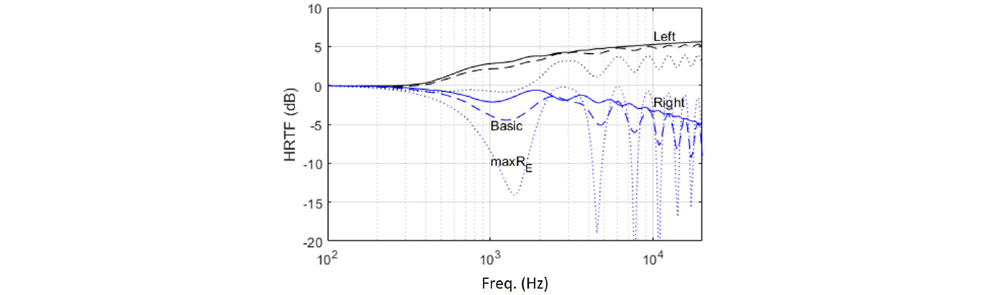
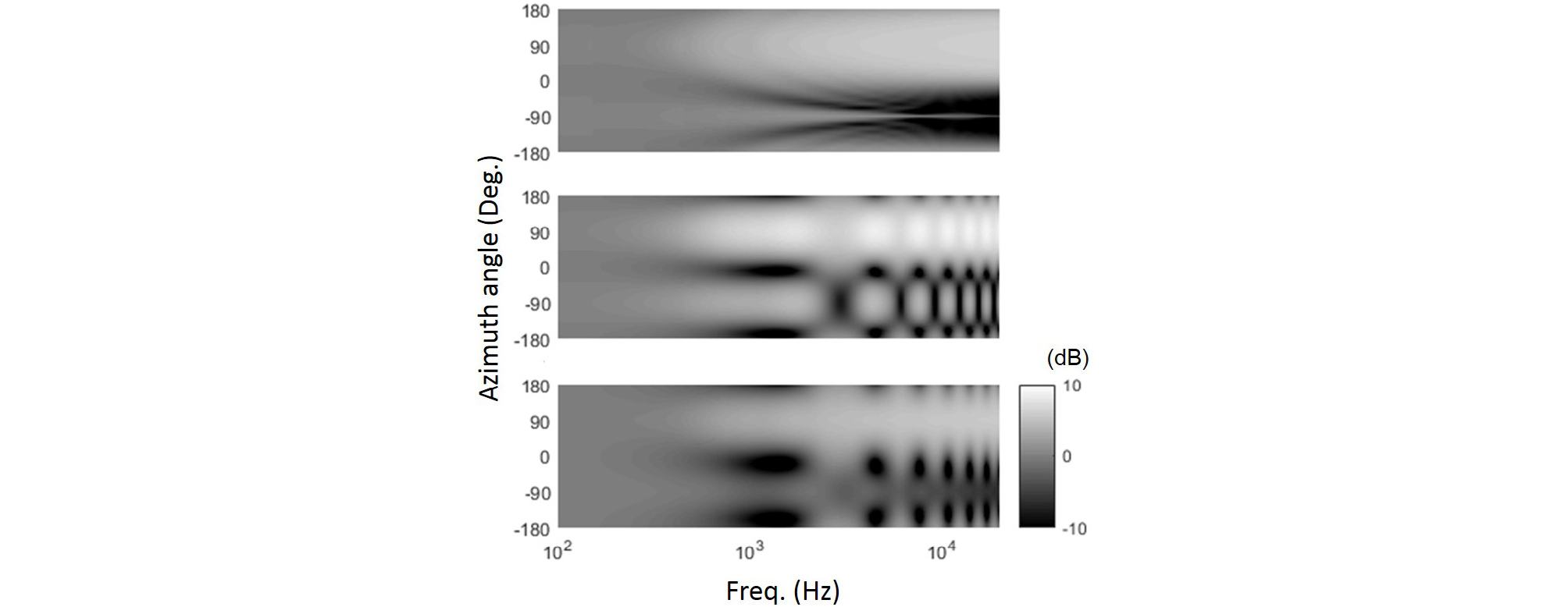
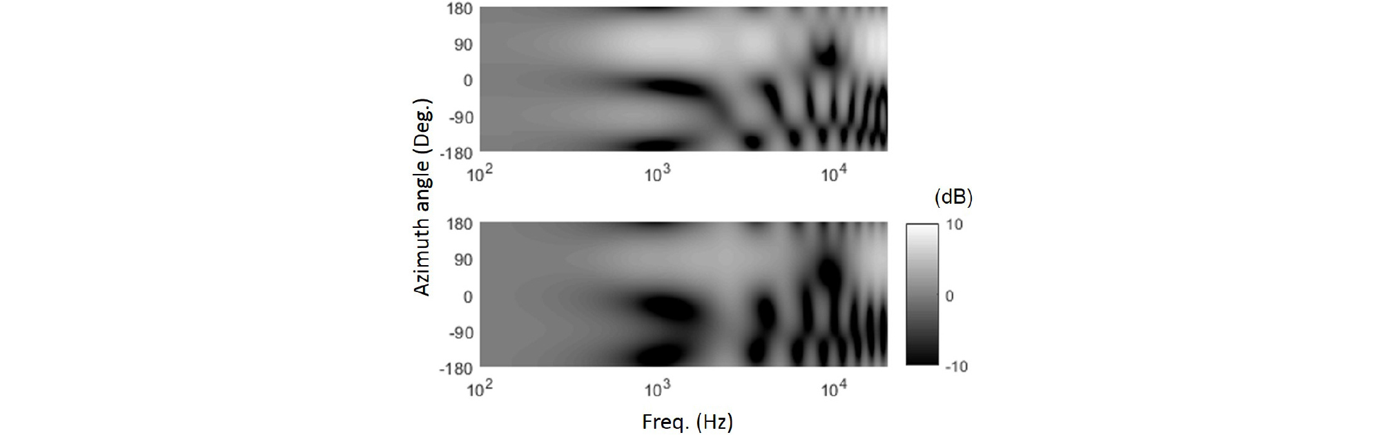
The reproduced HRTFs with virtual loudspeakers can be obtained as shown in Eq. (13). The reproduced HRTFs are denoted as and . For example, Fig. 1 shows true and reproduced HRTFs of a rigid sphere model for an incident plane wave propagating in (π/2, π/6). The layout #1 (Table 1) is used, so the number of virtual loudspeakers is 4. Solid lines are true HRTFs, dashed lines are reproduced HRTFs with the basic decoding, and dotted lines are reproduced with the max RE decoding. The true and the reproduced HRTFs have little difference at low frequencies up to 607 Hz, which is the maximum frequency for nearly perfect reproduction. However, above this frequency, both the reproduced HRTFs have fluctuations along frequency compared with true HRTFs. In this particular case, the magnitude of the reproduced HRTFs is smaller than that of the true HRTF in general, but it depends on the propagating direction of the incident wave. Fig. 2 shows left ear signal of true (top), reproduced HRTF with the basic decoding (middle) and the max RE (bottom) for different azimuth angles with the layout #1. Around -90 degree of the azimuth angle, the reproduced HRTF has fluctuation between ± 5 dB along the frequency, whilst the true HRTF has much lower values across the frequency. Fig. 3 also shows the left ear signal of reproduced HRTF but with the layout #2. The reproduced HRTFs have little difference from the true values [Fig. 2 (top)] only up to around 607 Hz, and above this frequency, the reproduced HRTF is not accurate either with the basic decoding or the max RE. The HRTF with the max RE (top) has smaller values than that with the basic decoding (bottom) in general. The results with the layout #3 are not shown because these results are identical to those with the layout #1. The reason is that these results are obtained only for plane waves propagating in the horizontal directions: the transfer functions of the loudspeakers in the upper positions (positive on z axis) and the lower positions (negative on z axis) are dependent at ear positions, and consequently the layout #1 and the layout #3 make no difference. For other propagating directions than the horizontal directions, there are differences between the layout #1 and #3. In what follows, results with the layout #3 are shown without those with the layout #1 and #2 because the layout #3 is the most widely used, and the differences are negligible or trivial. The effect of the layouts is discussed in Section 4.4.
A HRTF database that is measured with a mannequin with in-ear microphones is used in this study.[8] Fig. 4 shows true (solid lines) and reproduced (dotted lines) HRTF data by using this database for a plane wave propagating in (π/2, π/6). The layout #3 (Table 1) is used. The true and the reproduced data do not have a big difference up to around 607 Hz, but above this frequency, there are significant differences between those data. As a result, in the true HRTF data, the left ear signal has greater values than the right ear signal at all frequencies, but in the reproduced HRTF data, the left ear signal has smaller values than the right ear signal at some frequencies.

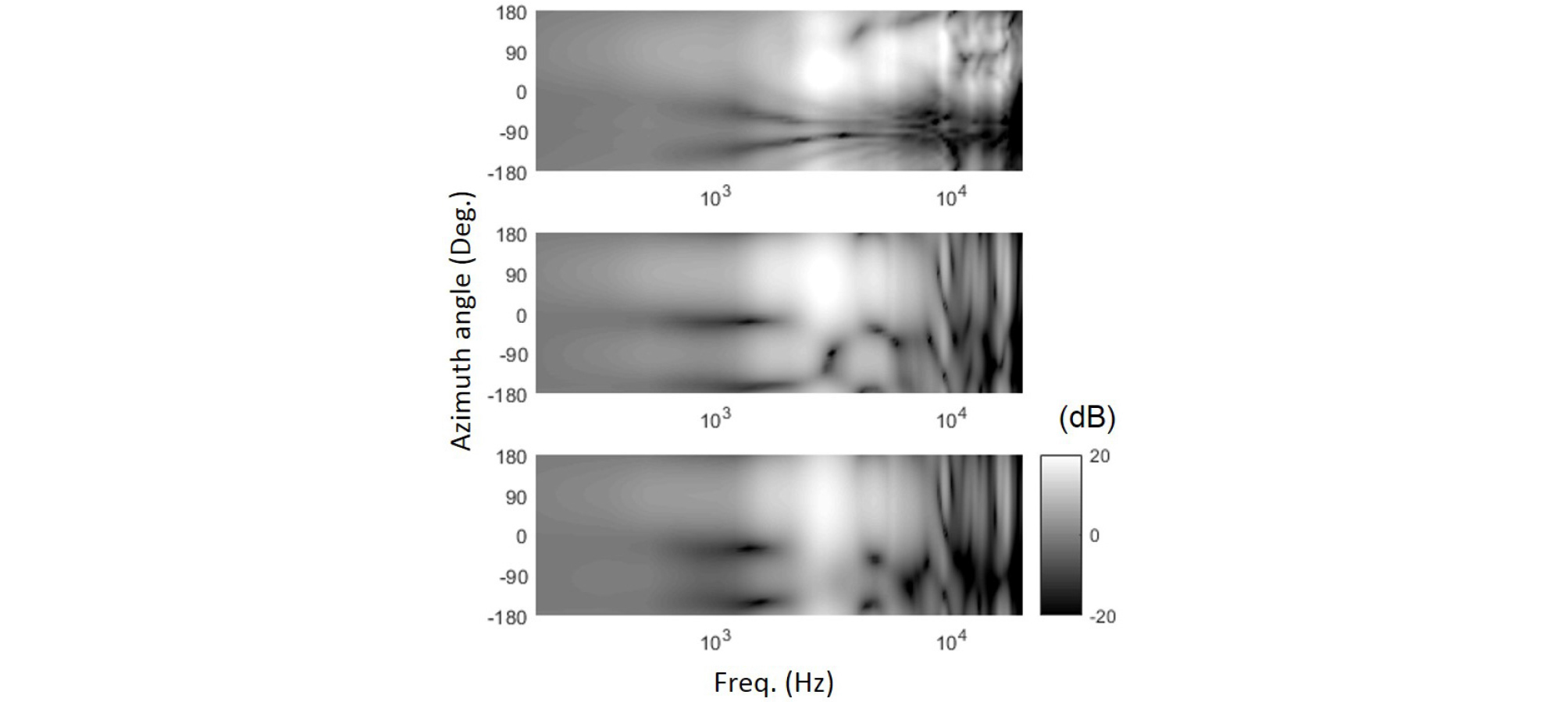
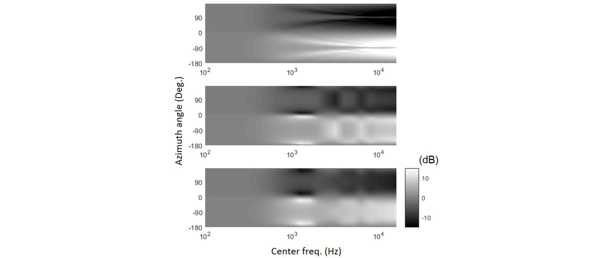
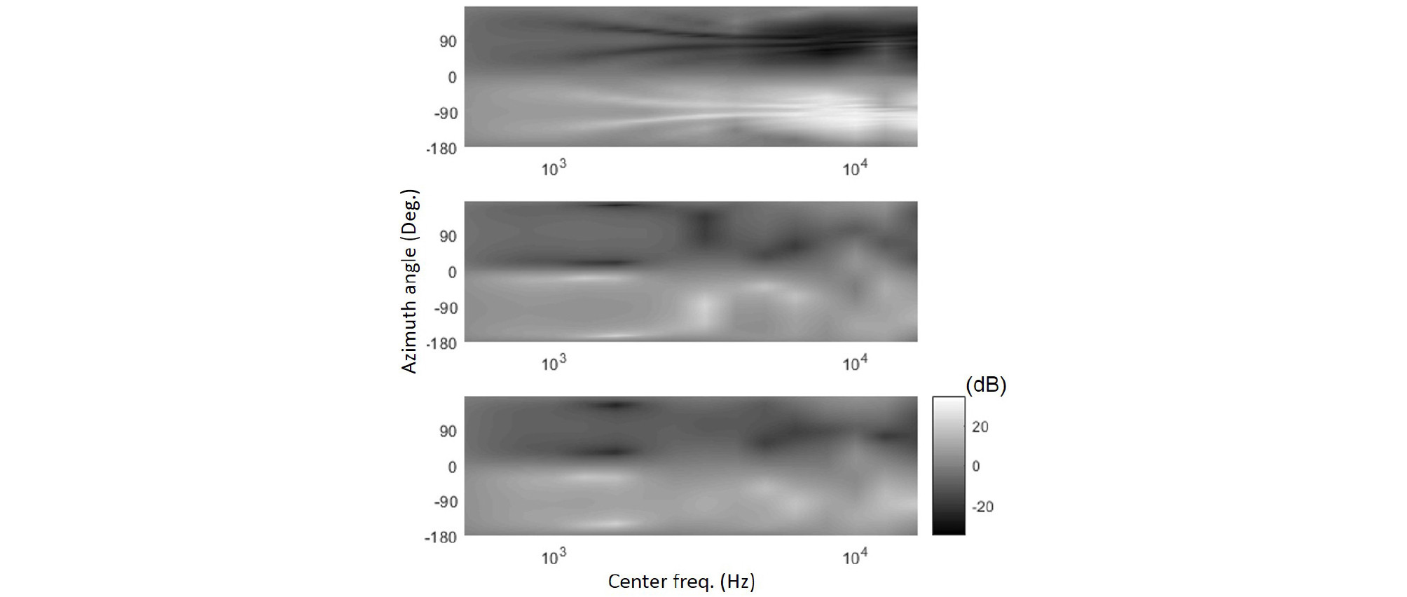
Fig. 5 shows true (top) and reproduced HRTF for the left ear with the basic decoding (middle) and the max RE (bottom) with respect to the azimuth angle. It can be clearly seen that at high frequencies above 10 kHz, the reproduced level is lower than the true level. In addition, there are two dark lines from about 1 kHz to 10 kHz that are symmetric to -90 degree in the top figure. These lines converge to -90 degree at high frequencies. However, in the middle and the bottom figures, these lines have discontinuity around 3 kHz, and do not converge to -90 degree. This difference affects the ILDs, which is discussed in Section 3.2.
In order to obtain the relative level [Eq. (9)], Eqs. (10), (13), and (19) are substituted into Eq. (14). Then, Eq. (14) can be reduced
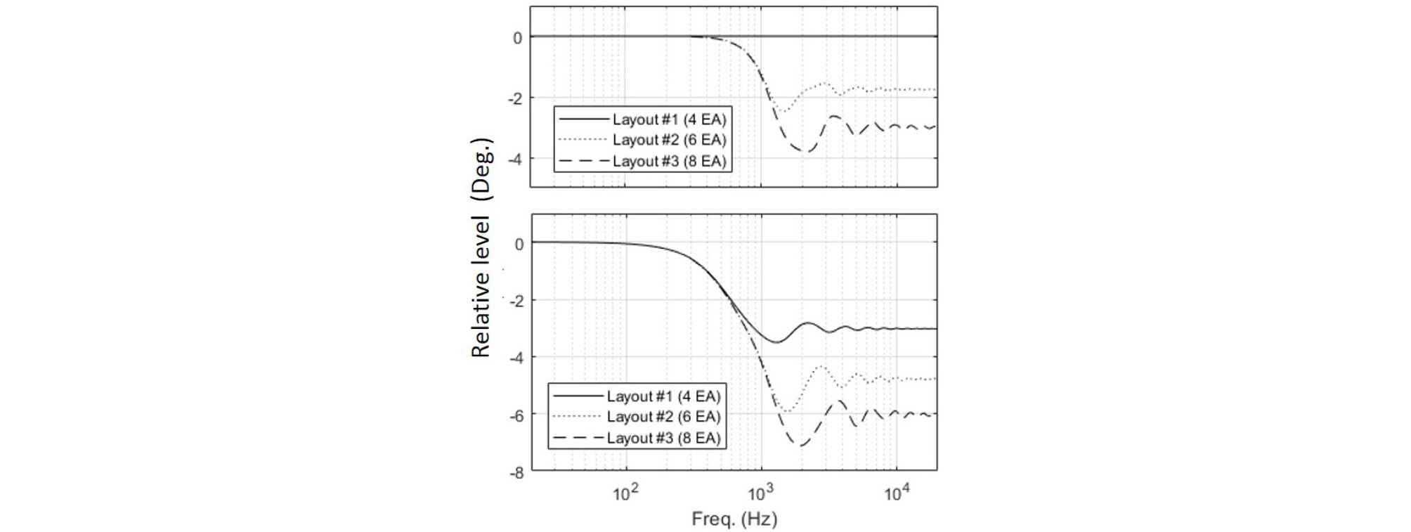
For the details, see Appendix. Fig. 6 shows the relative level averaged over the incident angle as shown in Eq. (14) with the basic decoding (top) and the max RE (bottom). The solid line, the dotted line, and the dashed line are the relative levels with 4, 6, and 8 virtual loudspeakers, respectively. In Fig. 6 (top), when the layout #1 is used, the relative level has no reduction. With the layout #2 and #3, the relative level begins to decrease from around 500 Hz, and fluctuate around a certain negative level at high frequencies. This means that the reproduced sound has spectral impairment above the frequency limit of nearly perfect reproduction. As the number of virtual loudspeakers increases, the relative level decreases more, and the fluctuation becomes bigger. In Fig. 6 (bottom), the relative levels have lower values at higher frequencies than 607 Hz. This means that the max RE leads to more reduction of the spectrum than the basic decoding does.
3.2 ILDs and IPDs for a source located in the horizontal plane
The ILDs [Eq. (15)] and the IPDs [Eq. (16)] are calculated by both the rigid sphere model and the database in each one third octave band. First, Figs. 7 and 8 show the ILDs and the IPDs by the rigid sphere model with the layout #3, respectively. The true ILD has smaller values at positive angles than those at negative angles. Positive angles indicate the left side, and thus the level at the left ear is greater than that at the right ear, which leads to smaller ILDs by the definition of ILDs [Eq. (15)].
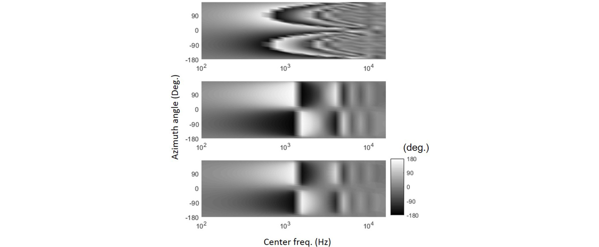
At low frequencies below 607 Hz, the ILDs have similar values in all the figures. The IPDs also have similar values to the true IPDs at these frequencies (Fig. 8). The ILD and IPD with the basic decoding have smaller error than those with the max RE decoding as shown in Fig. 9. In contrast, above 607 Hz, considerable differences between the true and the reproduced ILDs/IPDs are observed (Figs. 7 and 8). For example, at each frequency from 1 kHz to 20 kHz, the top figure in Fig. 7 has a local peak around 90 degree and a local dip around -90 degree, which can also be seen in Fig. 10. The width of these peaks and the dips decreases with the frequency. On the other hand, the middle and the bottom figures in Fig. 7 have relatively wide peaks and dips of which the width does not vary as much. At frequencies around 3 kHz and 6 kHz, the middle figure does not have such peaks and dips, and the bottom figure does not have at most frequencies above 2 kHz. Fig. 10 shows ILDs at 1.6 kHz and 8 kHz. In general, the ILD with the basic decoding has similar values to the true values at the dips (-90 degree) and at the peaks (90 degree), whilst the ILD with the max RE has similar values to the true values around 0 degree.
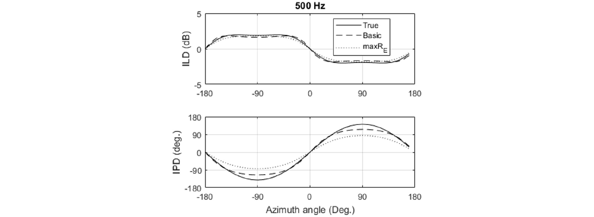
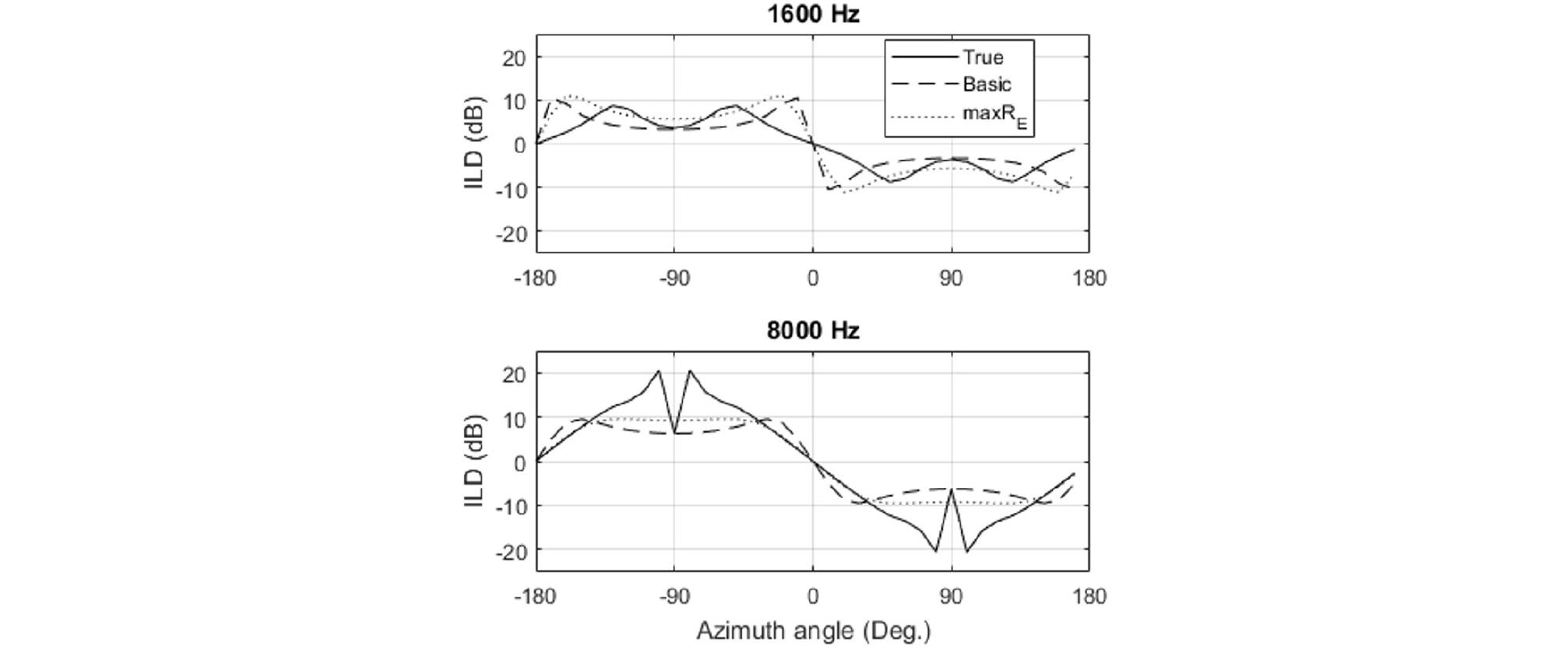
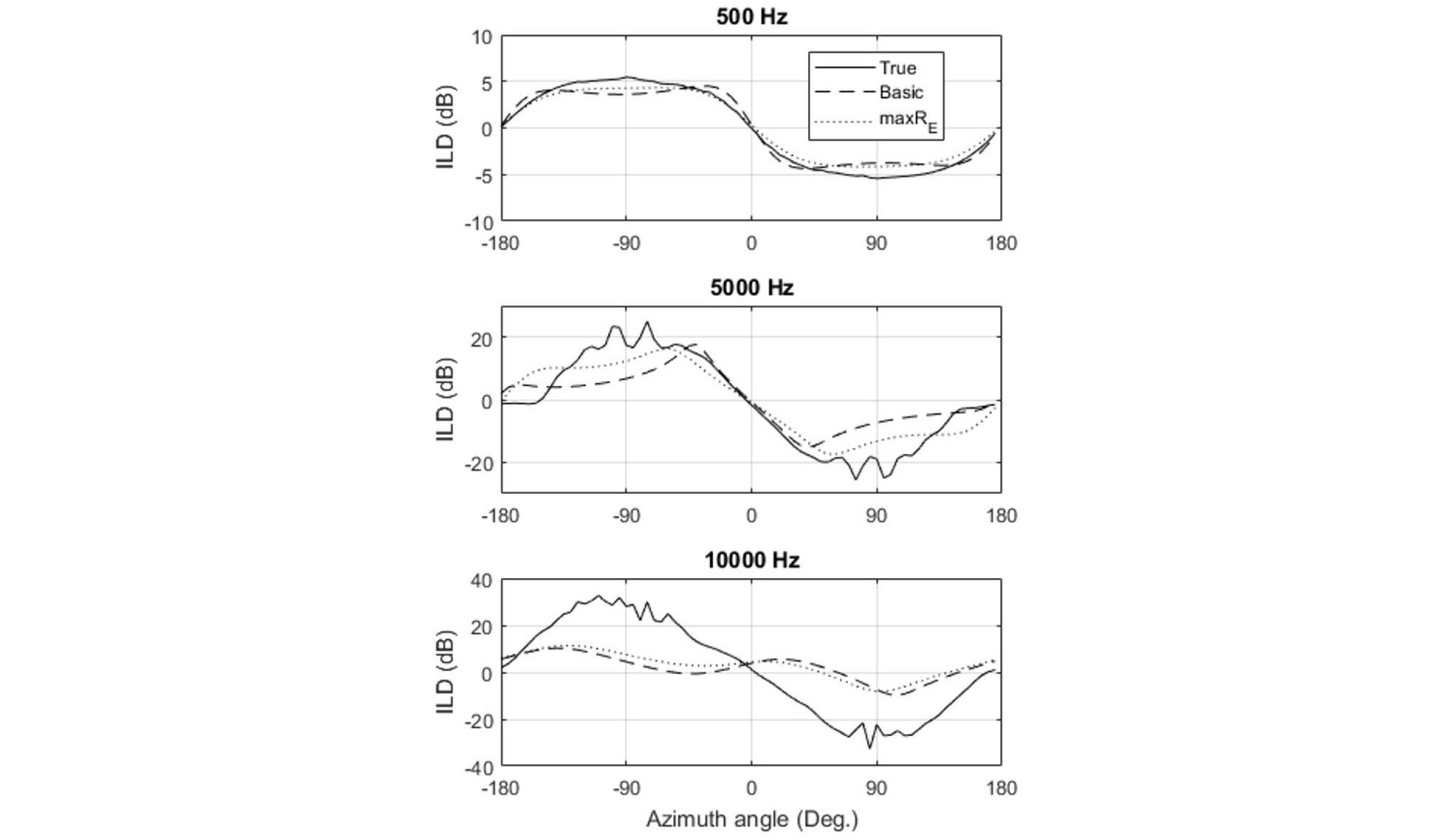
Fig. 11 shows the ILDs that are calculated with the measured HRTF database.[8] The magnitudes of the values are higher than those with the rigid sphere model (Fig. 7), but the same tendencies can be observed: the reproduction is accurate below 607 Hz, and significantly different at high frequencies. The local peaks and dips of which the widths decrease with the frequency can be seen from 1 kHz to 10 kHz only in the top figure. The ILDs with the max RE have similar values to the true values around the forward direction, 0 degree. This can be also seen in the top (500 Hz) and the middle figures (5 kHz) in Fig. 12. However, as shown in the bottom figure of Fig. 12, the reproduced ILDs are totally different from the true values at 10 kHz.
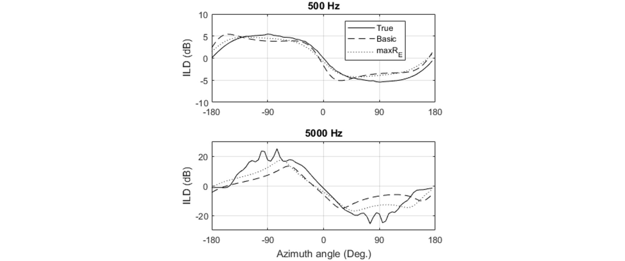
Although the ILDs and IPDs obtained with the layout #1 and #2 are not shown, when the layout #2 is used, the results were not so different from those with the layout #3. On the other hand, the results with the layout #1 have a significant difference when the measured HRTFs are used. Fig. 13 shows ILDs at 500 Hz and 5 kHz with the layout #1. Although the ILD should have a value of 0 dB at 0 degree of azimuth angle, and the ILD curves should be symmetric to the origin (0 degree, 0 dB) as the true ILD curve does, the ILD with the layout #1 has lower values than 0 dB at 0 degree, and the curve is not symmetric. It does not happen with the rigid sphere model that has no experimental noise (not shown).
IV. Discussions
4.1 Spectral compensation
As shown in Figs. 1 ~ 6, spectral impairment occurs above the cutoff frequency around 607 Hz. This impairment depends on the direction of incident waves as shown in Figs. 2, 3, and 6, and thus it could be compensated only if the direction is given. However, ambient sound includes sound waves from many different incident angles, and thus it cannot be individually compensated.
Instead, it is possible to compensate the resultant ear signals on average over the incident angle based on Fig. 6. That is, when the reproduction is conducted with 8 loudspeakers by the max RE, a high shelving filter that boosts about 6 dB at high frequencies can be applied. This simple compensation has an advantage that it could be more robust to individual differences such as the ear pinnae over the compensation based on the measured HRTF database.
4.2 Localization performance in the horizontal plane
Even though the cut off frequency of FOA is about 607 Hz, the ILDs around the forward direction have similar values to the true values. Since the ILD is a salient cue at high frequencies, listeners are likely to be able to localize the direction of the source around the forward direction. On the contrary, around ear positions, both the ILD and the IPD have considerable errors. Fortunately, the human ability of localizing sound source is also worse for these directions, and thus the performance degradation might not induce serious issues.
However, as shown in Fig. 12 (bottom), the ILD sometimes does not follow the true values even around the forward direction. In these cases, listeners might localize opposite directions, or confused by contradictory cues from different bands.
4.3 The effect of the decoding methods
Two decoding methods, the basic method and the max RE, were used to compare the results. In terms of the spectral distortion, the basic method has less reduction in the relative level as shown in Fig. 6. However, this reduction with the max RE is not too large to compensate. In terms of the localization performance in the horizontal plane, the basic method has more accurate ILDs and IPDs at low frequencies below the cutoff. At high frequencies, both methods fail, but the max RE has relatively more accurate ILDs around the forward direction in general. These results confirm what has been known in the previous studies,[3], [4] that the max RE improves the localization performance.
4.4 The effect of the layouts of loudspeakers
Three layouts were employed in this study as shown in Table 1. In terms of the spectral distortion, as more loudspeakers are used, the spectrum has the more reduction as shown in Fig. 6. When the number of loudspeakers is equal to that of the Ambisonic signals, which is 4, there was no distortion with the basic decoding in terms of the relative level. This result is consistent with what was found in,[20] although those results were obtained in two- dimensional case without considering the scattering effect of the user’s head.
As long as the rigid sphere model is used, the ILDs and the IPDs with the layout #1 have symmetric curves. But when the measured HRTFs are used, those with the layout #1 showed asymmetry as shown in Fig. 13. This means that the layout #1 is sensitive to experimental noise. The reproduced HRTFs with the layer #1 have differences between the left and the right ear signals even in the median plane although the azimuth angle is zero. Fig. 14 shows this difference with the true and the reproduced HRTFs by different layouts. Below 10 kHz, only those with the layout #1 have significant differences between the left and the right ear signals, and the differences with the other layouts are not greater than the true values. The asymmetrical arrangement of the layout #1 is likely to be the reason.

No significant difference has been found in the localization performances between the layout #2 and #3 in this study. It is not enough to conclude that the layout #3 is more stable than the layout #2.
V. Conclusions
This paper analyzed limitations of the binaural sound that is reproduced by FOA, which is widely used for virtual reality audio. The distortions in spectrum and sound localization in the horizontal plane were investigated by using the relative level averaged over the incident angle, the ILDs, and the IPDs.
The results show that (i) max RE leads to more reduction in the spectrum than the basic decoding at high frequencies, (ii) the ILDs and the IPDs are accurate with the basic decoding only below the cutoff frequencies, (iii) the ILDs and the IPDs with the max RE have relatively accurate values around the forward direction and inaccurate values around the ear directions in general, and (iv) the asymmetric loudspeaker layout (the layout #1) leads to different signals between the left and the right ears even when the azimuth angle of the desired sound wave is 0.
These results imply that spectral compensation (equalization) based on the relative level averaged over the incident angle (Fig. 4) could improve the quality of reproduced sound, and that the reproduction with FOA works only around the forward direction to some extent at most frequencies (above the cut off frequency). It might not be considerably noticeable because human localization ability also decreases for other directions than the forward.
This study also has some limitations: it was assumed that the Ambisonic signals have no errors. If a sound field is recorded by using sound field microphones, the distortions could be even bigger than what was shown in this study. In addition, listening tests were not conducted, and the localization performance in the median plane could not be analyzed.
Appendix
The denominator in Eq. (14), , is obtained by the integration of in Eq. (19). By substituting Eq. (19) into the numerator and replacing with ,
This can be reduced by the orthogonality of the spherical harmonics,
By the addition theorem,[36] it can be reduced as
In the similar way, the numerator can be expressed as follows
If the max RE is used, substitution of Eq. (10) leads to
Eq. (14) is obtained by dividing Eq. (A4) by Eq. (A3).
